
Notice
Recent Posts
Recent Comments
Link
| 일 | 월 | 화 | 수 | 목 | 금 | 토 |
|---|---|---|---|---|---|---|
| 1 | 2 | 3 | ||||
| 4 | 5 | 6 | 7 | 8 | 9 | 10 |
| 11 | 12 | 13 | 14 | 15 | 16 | 17 |
| 18 | 19 | 20 | 21 | 22 | 23 | 24 |
| 25 | 26 | 27 | 28 | 29 | 30 | 31 |
Tags
- level 1
- 파이썬
- SQL
- 데이터 분석
- seaborn
- 알고리즘
- Numpy
- 튜닝
- 실기
- 빅데이터 분석 기사
- level 2
- 프로그래머스
- Kaggle
- 실습
- 빅분기
- matplotlib
- 머신러닝
- R
- python3
- pandas
- Oracel
- Python
- 코딩테스트
- sklearn
- 오라클
- 카카오
- oracle
Archives
- Today
- Total
라일락 꽃이 피는 날
The Iris Dataset (4) - HDBSCAN 본문
728x90
HDBSCAN 알고리즘
[HDBSCAN 특징]
- DBSCAN에서 Hierarchical가 합쳐진 알고리즘
- different sizes, densities, noise, arbitrary shapes인 데이터에 적합
- 계층적 구조를 반영한 clustering 가능
1.다양한 분포와 사이즈의 데이터 생성
from sklearn.datasets import make_blobs# make_moons : 달 모양 군집 생성
# make_blobs : 원 모양 군집 생성
# centers 옵션으로 중심점 지정
# cluster_std 옵션으로 분포도 지정
moons, _ = make_moons(n_samples=100, noise=0.05)
blobs1, _ = make_blobs(n_samples=50, centers=[(-0.75, 2.25), (1.0, 2.0)], cluster_std=0.25)
blobs2, _ = make_blobs(n_samples=30, centers=[(-0.3, -1), (4.0, 1.5)], cluster_std=0.3)
blobs3, _ = make_blobs(n_samples=100, centers=[(3, -1), (4.0, 1.5)], cluster_std=0.4)
# 데이터를 하나로 합치기
hdb_data = np.vstack([moons, blobs1, blobs2, blobs3])
hdb_data_df = pd.DataFrame(hdb_data, columns=['x', 'y'])
hdb_data_df.head()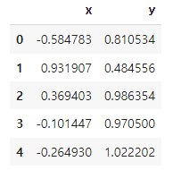
# scatter plot 그리기
fig = px.scatter(hdb_data_df, x='x', y='y')
fig.update_layout(width=600, height=500, title='HDBSCAN 데이터 분포')
fig.show()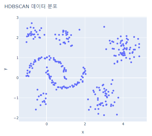
2. HDBSCAN 알고리즘 훈련
[HDBSCAN 파라미터]
- min_cluster_size (default=5) : 군집화를 위한 최소한의 cluster 사이즈
- min_samples (default=None) : 반경내 있어야할 최소 data points 수
- cluster_selection_epsilon(default=0.0) : 거리 기준, 기준 이하의 거리는 cluster끼리 merge
import hdbscanhdbscan_model = hdbscan.HDBSCAN(min_cluster_size=5)
hdbscan_model.fit(hdb_data)
# 훈련된 결과 label 확인
hdbscan_label = hdbscan_model.fit_predict(hdb_data)
set(hdbscan_label)  # {-1, 0, 1, 2, 3, 4, 5, 6}
3. HDBSCAN 알고리즘 파라미터 비교
# 훈련 결과를 plotly를 사용하여 시각화
hdb_data_df['hdbscan_label'] = hdbscan_label
hdb_data_df['hdbscan_label'] = hdb_data_df['hdbscan_label'].astype(str)

fig = px.scatter(hdb_data_df, x='x', y='y', color='hdbscan_label')
fig.update_layout(width=600, height=500)
fig.show()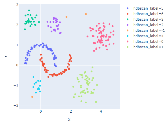
# min_cluster_size에 따른 clusters의 차이 비교
for mcn in [3,5,7,9,13]:
    hdbscan_label = hdbscan.HDBSCAN(min_cluster_size=mcn, min_samples=None, prediction_data=True).fit_predict(hdb_data)
    hdb_data_df['hdbscan_label'] = hdbscan_label
    hdb_data_df['hdbscan_label'] = hdb_data_df['hdbscan_label'].astype(str)

    hdbscan_case_dict = dict((x, list(hdbscan_label).count(x)) for x in set(hdbscan_label))
    if -1 in hdbscan_case_dict.keys():
        outliers = hdbscan_case_dict[-1]
    else:  # outlier가 없는 경우
        outliers = 0

    fig = px.scatter(hdb_data_df, x='x', y='y', color='hdbscan_label')
    fig.update_layout(width=600, height=500, title=f'min_cluster_size={mcn} >> label 수: {len(set(hdbscan_label))}, outlier: {outliers}')
    fig.show()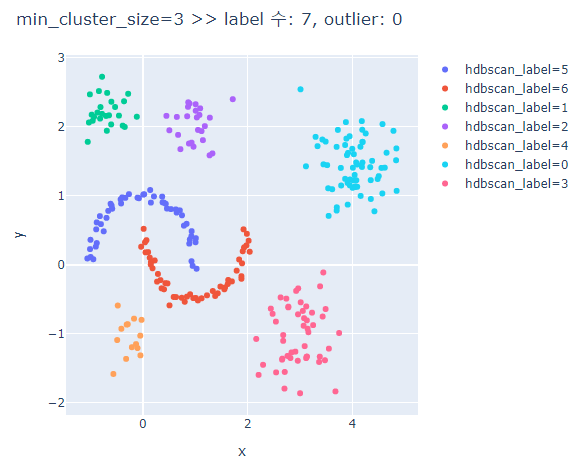
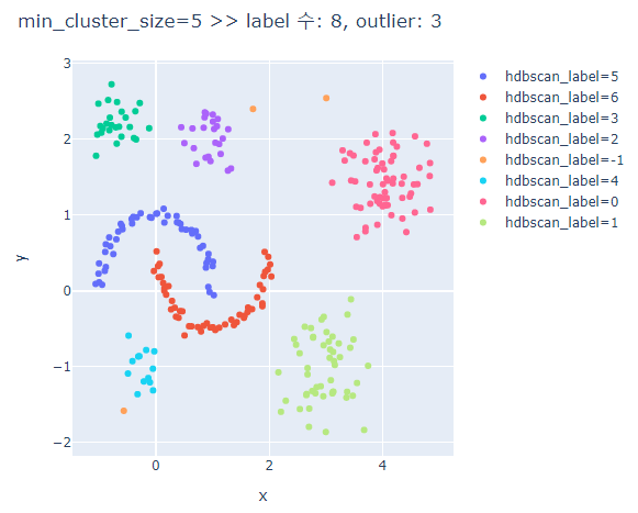
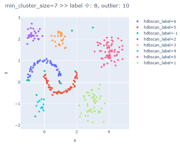
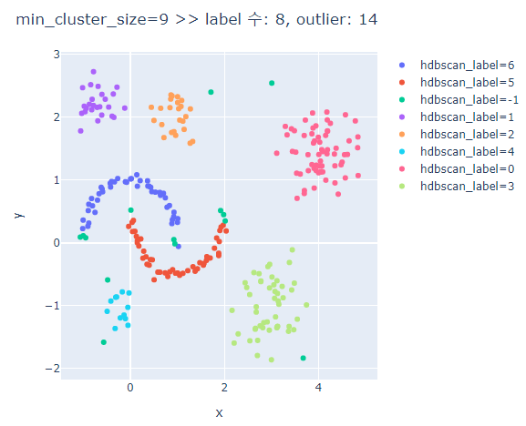
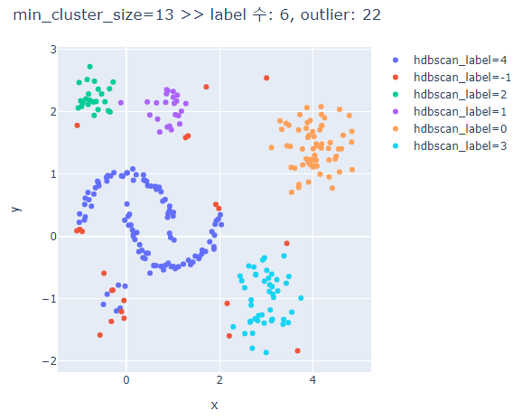
min_cluster_size가 커질수록 oulier가 많아진다.
min_cluster_size가 너무 크면 달 모형의 군집은 제대로 분류하지 못한다.
# min_samples에 따른 clusters의 차이 비교
for ms in [3,5,7,9,13]:
    hdbscan_label = hdbscan.HDBSCAN(min_cluster_size=5, min_samples=ms, prediction_data=True).fit_predict(hdb_data)
    hdb_data_df['hdbscan_label'] = hdbscan_label
    hdb_data_df['hdbscan_label'] = hdb_data_df['hdbscan_label'].astype(str)

    hdbscan_case_dict = dict((x, list(hdbscan_label).count(x)) for x in set(hdbscan_label))
    if -1 in hdbscan_case_dict.keys():
        outliers = hdbscan_case_dict[-1]
    else:  # outlier가 없는 경우
        outliers = 0

    fig = px.scatter(hdb_data_df, x='x', y='y', color='hdbscan_label')
    fig.update_layout(width=600, height=500, title=f'min_samples={ms} >> label 수: {len(set(hdbscan_label))}, outlier: {outliers}')
    fig.show()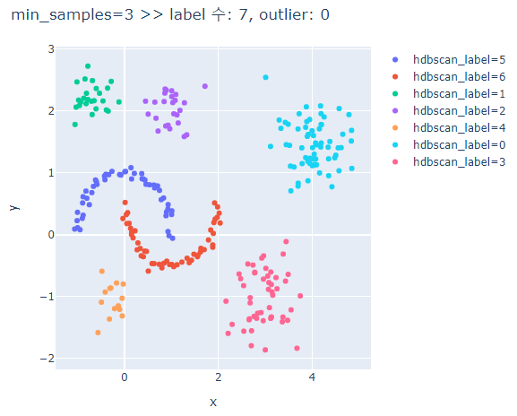

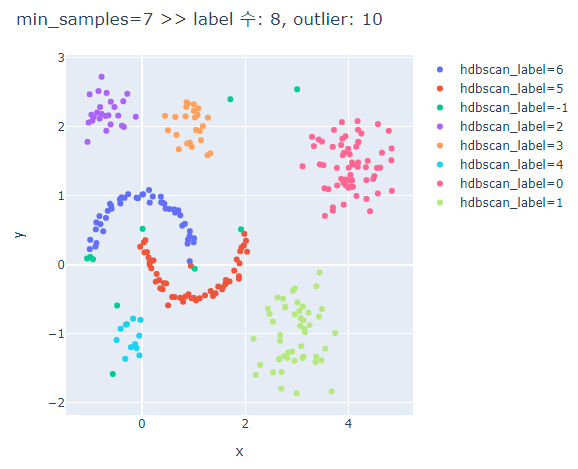
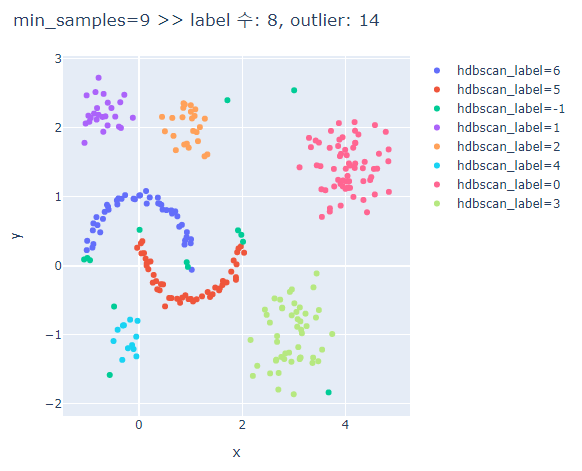
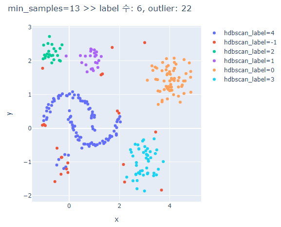
min_samples가 커질수록 oulier가 많아진다.
min_samples가 너무 크면 달 모형의 군집은 제대로 분류하지 못한다.
# cluster_selection_epsilon에 따른 clusters의 차이 비교
for cse in [0.1,0.5,0.7,1.0]:
    hdbscan_label = hdbscan.HDBSCAN(min_cluster_size=5, min_samples=None, cluster_selection_epsilon=cse, prediction_data=True).fit_predict(hdb_data)
    hdb_data_df['hdbscan_label'] = hdbscan_label
    hdb_data_df['hdbscan_label'] = hdb_data_df['hdbscan_label'].astype(str)

    hdbscan_case_dict = dict((x, list(hdbscan_label).count(x)) for x in set(hdbscan_label))
    if -1 in hdbscan_case_dict.keys():
        outliers = hdbscan_case_dict[-1]
    else:  # outlier가 없는 경우
        outliers = 0

    fig = px.scatter(hdb_data_df, x='x', y='y', color='hdbscan_label')
    fig.update_layout(width=600, height=500, title=f'cluster_selection_epsilon={cse} >> label 수: {len(set(hdbscan_label))}, outlier: {outliers}')
    fig.show()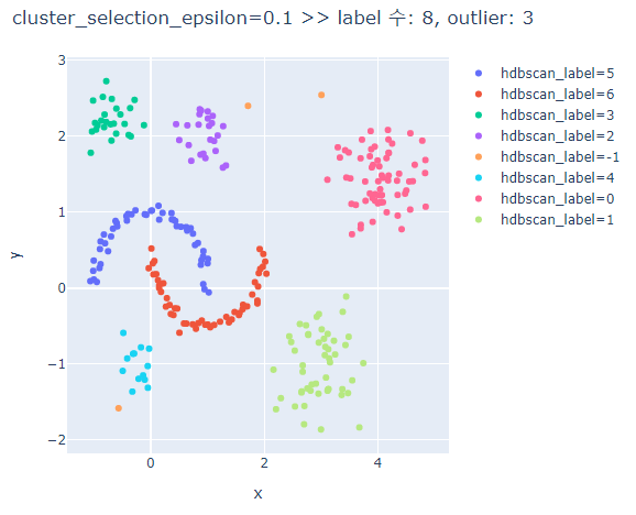
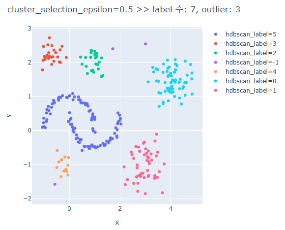
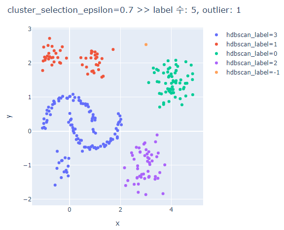
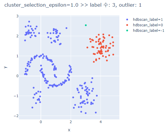
cluster_selection_epsilon가 클수록 하나의 군집으로 분류된다.
4. HDBSCAN의 다양한 시각화 확인
4-1. minimum_spanning_tree
- 각 point를 이어주는 line의 distance를 점수화한 mutual reachabillity를 사용하여 나타낸 그래프
- point간의 거리를 나타낸 것이 아닌, line을 그려나가면서 아직 추가되지 않은 point들 중에서 mutual reachabillity가 가장 낮은 point를 하나씩만 추가하는 방식으로 진행
# 시각화 생성을 위해 gen_min_span_tree=True로 훈련
hdbscan_model = hdbscan.HDBSCAN(min_cluster_size=5, min_samples=None, cluster_selection_epsilon=0.1, gen_min_span_tree=True).fit(hdb_data)

# 훈련된 모델을 사용하여 minimum_spanning_tree 생성
hdbscan_model.minimum_spanning_tree_.plot(edge_alpha=0.9, edge_cmap='viridis', node_size=10, edge_linewidth=1)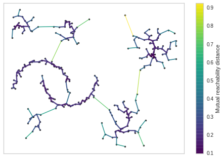
4-2. condensed_tree
- 가장 오래 버틴 cluster 순으로 cluster를 분류
# 훈련된 모델을 사용하여 condensed_tree 생성
# cluster도 함께 보기위해 select_clusters=True 설정
hdbscan_model.condensed_tree_.plot(select_clusters=True)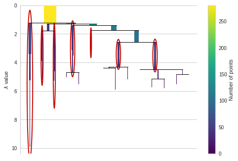
5. HDBSCAN와 K-means의 성능 비교
# k-means 훈련
hdb_data_km = KMeans(n_clusters=7).fit(hdb_data)

# hdbscan 훈련
hdb_data_hdbscan_label = hdbscan.HDBSCAN(min_cluster_size=5, min_samples=None, cluster_selection_epsilon=0.1, gen_min_span_tree=True).fit_predict(hdb_data)
hdb_data_df['kmeans_label'] = hdb_data_km.labels_
hdb_data_df['kmeans_label'] = hdb_data_df['kmeans_label'].astype(str)

hdb_data_df['hdbscan_label'] = hdb_data_hdbscan_label
hdb_data_df['hdbscan_label'] = hdb_data_df['hdbscan_label'].astype(str)
# plotly로 시각화하여 비교
for label_case in ['hdbscan_label', 'kmeans_label']:
    fig = px.scatter(hdb_data_df, x='x', y='y', color=label_case)
    fig.update_layout(width=600, height=500, title=f'{label_case} 시각화')
    fig.show()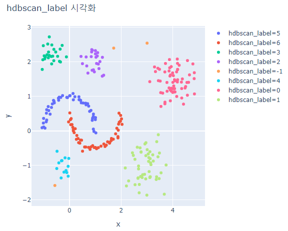
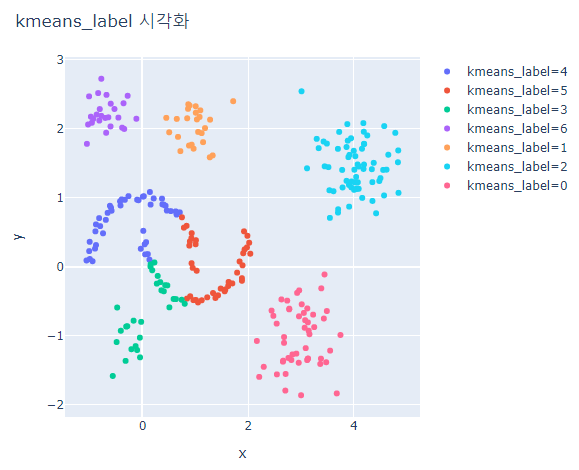
HDBSCAN은 대체적으로 잘 분류하지만 outlier가 발생한다.
K-means는 달 모형은 제대로 분류하지 못하지만 구 형태의 모형은 잘 분류한다.
6. HDBSCAN와 DBSCAN의 성능 비교
# dbscan 훈련
hdb_data_dbscan = DBSCAN(eps=0.3, min_samples=5).fit(hdb_data)

hdb_data_df['dbscan_label'] = hdb_data_dbscan
hdb_data_df['dbscan_label'] = hdb_data_df['dbscan_label'].astype(str)
# plotly로 시각화하여 비교
for label_case in ['hdbscan_label', 'dbscan_label']:
fig = px.scatter(hdb_data_df, x='x', y='y', color=label_case)
fig.update_layout(width=600, height=500, title=f'{label_case} 시각화')
fig.show()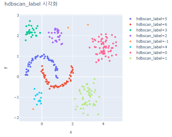
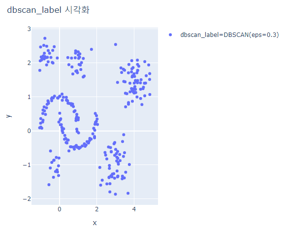
HDBSCAN은 대체적으로 잘 분류하지만 outlier가 발생한다.
DBSCAN은 모두 하나의 cluster로 분류되었다.
7. 데이터 분포에 따른 HDBSCAN와 DBSCAN의 차이 확인
# HDBSCAN와 DBSCAN을 비교할 분산이 극단적인 두가지 케이스의 데이터 생성
blobs1, _ = make_blobs(n_samples=200, centers=[(-10, 5), (0, -5)], cluster_std=0.5)
blobs2, _ = make_blobs(n_samples=200, centers=[(30, -1), (30, 1.5)], cluster_std=5.0)

comp_data = np.vstack([blobs1, blobs2])
comp_data_df = pd.DataFrame(comp_data, columns=['x', 'y'])
comp_data_df.head()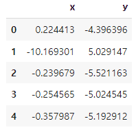
# scatter plot 그리기
fig = px.scatter(comp_data_df, x='x', y='y')
fig.update_layout(width=600, height=500, title='데이터 분포')
fig.show()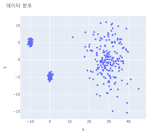
# dbscan 훈련
dbscan_model = DBSCAN(eps=0.6, min_samples=10).fit(comp_data)
comp_data_df["dbscan_label"] = dbscan_model.labels_
comp_data_df["dbscan_label"] = comp_data_df["dbscan_label"].astype(str)

# hdbscan 훈련
hdbscan_lables = hdbscan.HDBSCAN(min_cluster_size=5, min_samples=None, cluster_selection_epsilon=0.1, gen_min_span_tree=True).fit_predict(comp_data)
comp_data_df["hdbscan_label"] = hdbscan_lables
comp_data_df["hdbscan_label"] = comp_data_df["hdbscan_label"].astype(str)
# outlier를 구분하기 위한 color 컬럼 생성
color_dict = {"-1":"#d8d8d8", "0":"#ff5e5b", "1":"#457b9d", "2":"#00cecb", "3":"#FFED66"}
comp_data_df['dbscan_label_color'] = comp_data_df['dbscan_label'].map(color_dict)
comp_data_df['hdbscan_label_color'] = comp_data_df['hdbscan_label'].map(color_dict)
# 두 모델 결과를 시각화로 나타내고 차이가 나타나는지 확인
for label_case in ['hdbscan_label_color', 'dbscan_label_color']:
    fig = go.Figure(data=go.Scatter(
        x = comp_data_df['x'],
        y = comp_data_df['y'],
        mode = 'markers',
        marker = dict(color=comp_data_df[label_case], showscale=True)
    ))
    fig.update_layout(width=600, height=500, title=f'{label_case} 시각화')
    fig.show()
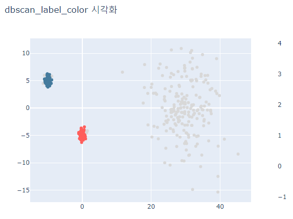
회색으로 나타나는 point는 outlier로 분류된 points이다.
HDBSCAN은 분산이 작은 데이터와 큰 데이터 모두 잘 분류한다.
DBSCAN은 분산이 큰 데이터는 분류하지 못하고 oulier로 취급한다.
728x90
'데이터 분석 > 실습' 카테고리의 다른 글
| The Iris Dataset (3) - DBSCAN (0) | 2022.01.19 |
|---|---|
| The Iris Dataset (2) - Agglomerative (0) | 2022.01.19 |
| The Iris Dataset (1) - K-Means (0) | 2022.01.18 |
| COVID-19 data from John Hopkins University (0) | 2022.01.06 |
| Video Game Sales with Ratings (0) | 2022.01.06 |
'데이터 분석/실습' Related Articles
more


