
Notice
Recent Posts
Recent Comments
Link
| 일 | 월 | 화 | 수 | 목 | 금 | 토 |
|---|---|---|---|---|---|---|
| 1 | 2 | 3 | ||||
| 4 | 5 | 6 | 7 | 8 | 9 | 10 |
| 11 | 12 | 13 | 14 | 15 | 16 | 17 |
| 18 | 19 | 20 | 21 | 22 | 23 | 24 |
| 25 | 26 | 27 | 28 | 29 | 30 | 31 |
Tags
- sklearn
- SQL
- 실습
- 카카오
- 알고리즘
- 데이터 분석
- Oracel
- R
- 코딩테스트
- 프로그래머스
- python3
- level 2
- 빅분기
- 머신러닝
- 파이썬
- Kaggle
- pandas
- seaborn
- oracle
- 실기
- 튜닝
- Numpy
- 오라클
- 빅데이터 분석 기사
- matplotlib
- Python
- level 1
Archives
- Today
- Total
라일락 꽃이 피는 날
The Iris Dataset (2) - Agglomerative 본문
728x90
Clustering : Agglomerative 알고리즘 (계층군집)
[Hierarchical clustering 장점]
- cluster 수(k)를 정하지 않아도 사용 가능
- random point에서 시작하지 않으므로 동일한 결과가 나옴
- dendrogram을 통해 전체적인 군집 확인 가능 (nested clusters)
[Hierarchical clustering 단점]
- 대용량 데이터는 계산이 많아서 비효율적
1. Agglomerative 모듈 훈련
[AgglomerativeClustering 파라미터 참고사항]
- linkage 종류 : {‘ward’, ‘complete’, ‘average’, ‘single’}
- linkage="ward"이면, affinity="euclidean"
- distance_threshold!=None 이면, n_clusters=None
- distance_threshold!=None 이면, compute_full_tree=True
from sklearn.cluster import AgglomerativeClusteringaggl = AgglomerativeClustering(n_clusters=3, linkage='ward', affinity='euclidean').fit(train_x)
aggl_labels = aggl.labels_
2. 훈련된 cluster를 그래프로 비교
# 실제 label과 훈련된 결과 cluster를 그래프로 비교
fig = make_subplots(rows=1, cols=2, subplot_titles=('actual', 'aggl cluster'))

fig.add_trace(
    go.Scatter(x=train_x['sepal_width'],
               y=train_x['sepal_length'],
               mode='markers',
               marker=dict(color=train_y)),
    row=1, col=1
)

fig.add_trace(
    go.Scatter(x=train_x['sepal_width'],
               y=train_x['sepal_length'],
               mode='markers',
               marker=dict(color=aggl_labels)),
    row=1, col=2
)

fig.update_layout(width=800, height=600)
fig.show()
Agglomerative 모듈로 훈련한 결과, 실제 label과 유사한 분포를 보인다.
그러나 실제 cluster명과 완전히 매칭되지 않는다.
fig = make_subplots(rows=1, cols=2, subplot_titles=('actual', 'aggl cluster'))

fig.add_trace(
    go.Scatter(x=train_x['petal_width'],
               y=train_x['petal_length'],
               mode='markers',
               marker=dict(color=train_y)),
    row=1, col=1
)

fig.add_trace(
    go.Scatter(x=train_x['petal_width'],
               y=train_x['petal_length'],
               mode='markers',
               marker=dict(color=aggl_labels)),
    row=1, col=2
)

fig.update_layout(width=800, height=600)
fig.show()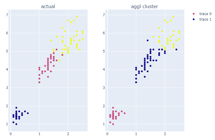
Agglomerative 모듈로 훈련한 결과, 실제 label과 유사한 분포를 보인다.
그러나 실제 cluster명과 완전히 매칭되지 않는다.
3. clustering 결과를 수치적으로 평가
# label 종류 저장
aggl_case = list(set(aggl_labels))
print(aggl_case)  # [0, 1, 2]

# find_matching_cluster 함수를 사용하여 매칭되는 dictionary 생성
aggl_perm_dict = find_matching_cluster(aggl_case, train_y, aggl_labels)
print(aggl_perm_dict)

# 생성한 dict 변수를 사용하여 훈련된 결과 label 변경
aggl_new_labels = [aggl_perm_dict[label] for label in aggl_labels]
# 새로 할당된 cluster명으로 accuracy score 계산
aggl_acc = accuracy_score(train_y, aggl_new_labels)
aggl_acc  # 0.883333
정확도 = 0.8833333
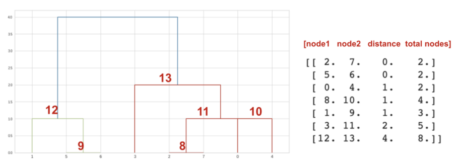
4. dendrogram을 그리기 위한 linkage matrix 구성 이해
from matplotlib import pyplot as plt
from scipy.cluster.hierarchy import dendrogram, linkage
# 샘플 데이터를 통해 linkage matrix 구조 파악
sample_arr = [[i] for i in [2, 8, 0, 4, 1, 9, 9, 0]]
sample_arr # [[2], [8], [0], [4], [1], [9], [9], [0]]
# 샘플 데이터로 linkage matrix 생성
sample_linkage = linkage(sample_arr, 'single')
print(sample_linkage)
# linkage matrix를 사용하여 dendrogram 그리기
fig = plt.figure(figsize=(13, 6))
dh = dendrogram(sample_linkage)
plt.show()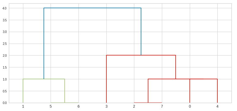
5. dendrogram을 통해 알고리즘 이해
# linkage_matrix를 생성하는 함수 생성
def create_linkage(model):
  # 각 노드에 총 point수 계산
  counts = np.zeros(model.children_.shape[0])  # children 길이만큼 0 채운 array
  n_samples = len(model.labels_)  # 각 point의 cluster label

  for i, merge in enumerate(model.children_):
    current_count = 0
    for child_idx in merge:
      if child_idx < n_samples:
        current_count += 1  # leaf node
      else:
        current_count += counts[child_idx - n_samples]
    counts[i] = current_count

  linkage_matrix = np.column_stack([model.children_, model.distances_, counts]).astype(float)
  return linkage_matrix
# Dendrogram을 그리기 위해서 distance_threshold와 n_clusters 파라미터 조정 필요
aggl_dend = AgglomerativeClustering(n_clusters=None, distance_threshold=0).fit(train_x)
# create_linkage 함수를 사용하여 linkage matrix를 생성하고 dendrogram 그리기
# x축: 실제 point (혹은 각 노드에 포함되는 point 수)
plt.title('Agglomerative Clustering Dendrogram')
linkage_matrix = create_linkage(aggl_dend)
dendrogram(linkage_matrix, truncate_mode='level', p=3)
plt.show()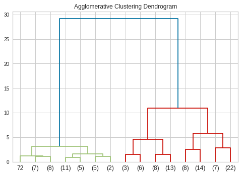
dendrogram을 보면 cluster를 4개로 나누는 것이 적합하다.
# dendrogram에서 정한 cluster 수로 모델 훈련
aggl = AgglomerativeClustering(n_clusters=4, linkage='ward', affinity='euclidean').fit(train_x)

aggl_labels = aggl.labels_
# 실제 label과 훈련된 결과 cluster를 그래프로 비교
fig = make_subplots(rows=1, cols=2, subplot_titles=('actual', 'aggl cluster'))

fig.add_trace(
    go.Scatter(x=train_x['sepal_width'],
               y=train_x['sepal_length'],
               mode='markers',
               marker=dict(color=train_y)),
    row=1, col=1
)

fig.add_trace(
    go.Scatter(x=train_x['sepal_width'],
               y=train_x['sepal_length'],
               mode='markers',
               marker=dict(color=aggl_labels)),
    row=1, col=2
)

fig.update_layout(width=800, height=600)
fig.show()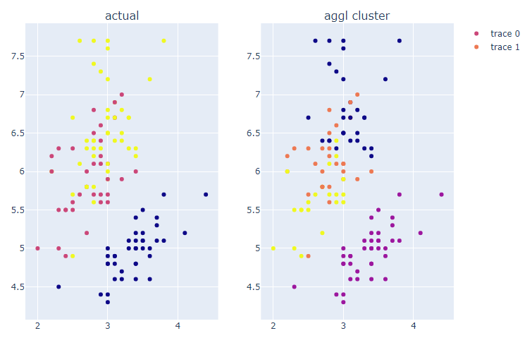
꽃받침의 폭이 좁고 길이가 긴 그룹이 더 세분화되어 나뉘어졌다.
fig = make_subplots(rows=1, cols=2, subplot_titles=('actual', 'aggl cluster'))

fig.add_trace(
    go.Scatter(x=train_x['petal_width'],
               y=train_x['petal_length'],
               mode='markers',
               marker=dict(color=train_y)),
    row=1, col=1
)

fig.add_trace(
    go.Scatter(x=train_x['petal_width'],
               y=train_x['petal_length'],
               mode='markers',
               marker=dict(color=aggl_labels)),
    row=1, col=2
)

fig.update_layout(width=800, height=600)
fig.show()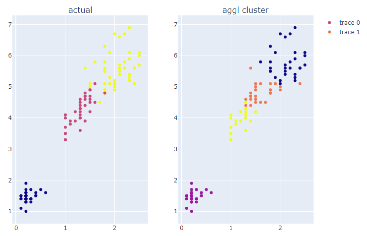
꽃잎의 폭이 넓고 길이가 긴 그룹이 더 세분화되어 나뉘어졌다.
728x90
'데이터 분석 > 실습' 카테고리의 다른 글
| The Iris Dataset (4) - HDBSCAN (0) | 2022.01.20 |
|---|---|
| The Iris Dataset (3) - DBSCAN (0) | 2022.01.19 |
| The Iris Dataset (1) - K-Means (0) | 2022.01.18 |
| COVID-19 data from John Hopkins University (0) | 2022.01.06 |
| Video Game Sales with Ratings (0) | 2022.01.06 |
'데이터 분석/실습' Related Articles
more


