
| 일 | 월 | 화 | 수 | 목 | 금 | 토 |
|---|---|---|---|---|---|---|
| 1 | 2 | 3 | ||||
| 4 | 5 | 6 | 7 | 8 | 9 | 10 |
| 11 | 12 | 13 | 14 | 15 | 16 | 17 |
| 18 | 19 | 20 | 21 | 22 | 23 | 24 |
| 25 | 26 | 27 | 28 | 29 | 30 | 31 |
- pandas
- R
- python3
- oracle
- Numpy
- 튜닝
- matplotlib
- SQL
- Kaggle
- Python
- 실습
- Oracel
- 프로그래머스
- 빅분기
- 코딩테스트
- 실기
- 파이썬
- level 2
- sklearn
- 머신러닝
- 빅데이터 분석 기사
- 오라클
- 카카오
- level 1
- 데이터 분석
- 알고리즘
- seaborn
- Today
- Total
라일락 꽃이 피는 날
Used Cars 본문
- id : 중고차 거래의 아이디
- url : 중고차 거래 페이지
- region : 해당 거래의 관리 지점
- region_url : 거래 관리 지점의 홈페이지
- price : 기입된 자동차의 거래가
- year : 거래가 기입된 년도
- manufacturer : 자동차를 생산한 회사
- model : 자동차 모델
- condition : 자동차의 상태
- cylinders : 자동차의 기통 수
- fuel : 자동차의 연료 타입
- odometer : 자동차의 운행 마일 수
- title_status : 자동차의 타이틀 상태 (소유주 등록 상태)
- transmission : 자동차의 트랜스미션 종류
- vin : 자동차의 식별 번호 (vehicle identification number)
- drive : 자동차의 구동 타입
- size : 자동차 크기
- type : 자동차의 일반 타입
- paint_color : 자동차 색상
- image_url : 자동차 이미지
- description : 세부 설명
- county : 실수로 생성된 미사용 컬럼
- state : 거래가 업로드된 미 주
- lat : 거래가 업로드된 곳의 위도
- long : 거래가 업로드된 곳의 경도
데이터셋 준비
import pandas as pd
import numpy as np
import matplotlib.pyplot as plt
import seaborn as sns
df = pd.read_csv('../input/craigslist-carstrucks-data/vehicles.csv')EDA 및 데이터 기초 통계 분석
df.head()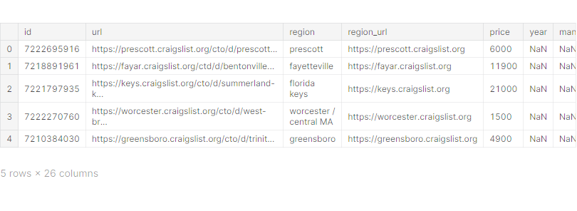
수치형 데이터: year, odometer, lat, long
범주형 데이터: id, url, region, region_url, manufacturer, model, codition, cylinders, fuel, title_status, transmission, VIN, drive, size, type, paint_color, image_url, description, state, posting_date
타겟 데이터: price
df.info()<class 'pandas.core.frame.DataFrame'>
RangeIndex: 426880 entries, 0 to 426879
Data columns (total 26 columns):
# Column Non-Null Count Dtype
--- ------ -------------- -----
0 id 426880 non-null int64
1 url 426880 non-null object
2 region 426880 non-null object
3 region_url 426880 non-null object
4 price 426880 non-null int64
5 year 425675 non-null float64
6 manufacturer 409234 non-null object
7 model 421603 non-null object
8 condition 252776 non-null object
9 cylinders 249202 non-null object
10 fuel 423867 non-null object
11 odometer 422480 non-null float64
12 title_status 418638 non-null object
13 transmission 424324 non-null object
14 VIN 265838 non-null object
15 drive 296313 non-null object
16 size 120519 non-null object
17 type 334022 non-null object
18 paint_color 296677 non-null object
19 image_url 426812 non-null object
20 description 426810 non-null object
21 county 0 non-null float64
22 state 426880 non-null object
23 lat 420331 non-null float64
24 long 420331 non-null float64
25 posting_date 426812 non-null object
dtypes: float64(5), int64(2), object(19)
memory usage: 84.7+ MB
(426880, 26) → 426880 rows 26 columns
county 컬럼에는 데이터가 없다. → 미사용 컬럼
df.isna().sum()id 0
url 0
region 0
region_url 0
price 0
year 1205
manufacturer 17646
model 5277
condition 174104
cylinders 177678
fuel 3013
odometer 4400
title_status 8242
transmission 2556
VIN 161042
drive 130567
size 306361
type 92858
paint_color 130203
image_url 68
description 70
county 426880
state 0
lat 6549
long 6549
posting_date 68
dtype: int64id, url, region, region_url, price, state 를 제외한 컬럼들에 null 값이 존재한다.
df.describe()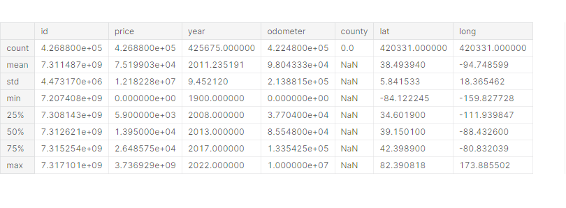
가격의 min, max 값이 비정상적으로 보인다 → outlier
가격의 평균값과 50% 값의 차이가 매우 크다.
최소 거래 년도가 1900년인 것으로 보아 기본 값으로 추정된다 → outlier
df.columnsIndex(['id', 'url', 'region', 'region_url', 'price', 'year', 'manufacturer',
'model', 'condition', 'cylinders', 'fuel', 'odometer', 'title_status',
'transmission', 'VIN', 'drive', 'size', 'type', 'paint_color',
'image_url', 'description', 'county', 'state', 'lat', 'long',
'posting_date'],
dtype='object')# 데이터프레임에서 불필요한 컬럼 제거
df.drop(['id', 'url', 'region_url', 'VIN', 'description',
'county', 'state', 'lat', 'long', 'posting_date'],
axis=1, inplace=True)
# 'year' 컬럼을 'age' 컬럼으로 변경
df['age'] = 2021 - df['year']
df.drop('year', axis=1, inplace=True)
df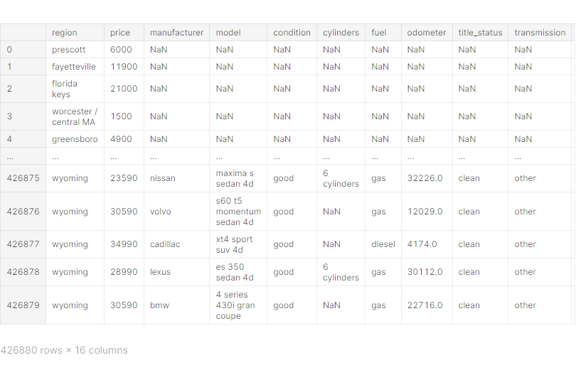
df['manufacturer'].value_counts()ford 70985
chevrolet 55064
toyota 34202
honda 21269
nissan 19067
jeep 19014
ram 18342
gmc 16785
bmw 14699
dodge 13707
mercedes-benz 11817
hyundai 10338
subaru 9495
volkswagen 9345
kia 8457
lexus 8200
audi 7573
cadillac 6953
chrysler 6031
acura 5978
buick 5501
mazda 5427
infiniti 4802
lincoln 4220
volvo 3374
mitsubishi 3292
mini 2376
pontiac 2288
rover 2113
jaguar 1946
porsche 1384
mercury 1184
saturn 1090
alfa-romeo 897
tesla 868
fiat 792
harley-davidson 153
ferrari 95
datsun 63
aston-martin 24
land rover 21
morgan 3
Name: manufacturer, dtype: int64
# seaborn의 countplot()로 범주별 통계 그리기
# order 옵션으로 출력 순서 지정
fig = plt.figure(figsize=(8, 10))
sns.countplot(y='manufacturer', data=df.fillna('n/a'), order=df.fillna('n/a')['manufacturer'].value_counts().index)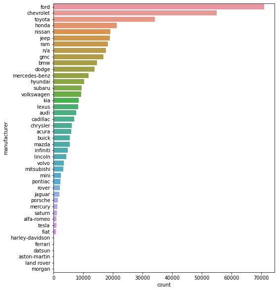
자동차를 생산한 회사는 ford가 가장 많다.
df['model'].value_counts()f-150 8009
silverado 1500 5140
1500 4211
camry 3135
silverado 3023
...
Huyndai Sante Fe Limited 1
astro awd 4x4 1
escalade and 1
cx 3 1
Paige Glenbrook Touring 1
Name: model, Length: 29667, dtype: int64
sns.countplot(y='condition', data=df.fillna('n/a'), order=df.fillna('n/a')['condition'].value_counts().index)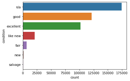
자동차의 상태는 null 값이 가장 많고, 다음으로 good이 많다.
sns.countplot(y='cylinders', data=df.fillna('n/a'), order=df.fillna('n/a')['cylinders'].value_counts().index)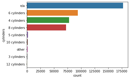
자동차의 기통 수는 null 값이 가장 많고, 다음으로 6기통이 많다.
sns.countplot(y='fuel', data=df.fillna('n/a'), order=df.fillna('n/a')['fuel'].value_counts().index)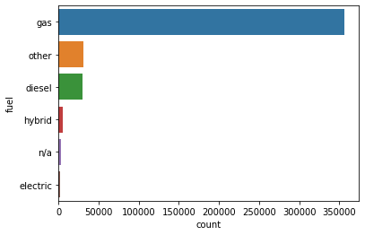
자동차의 연료 타입은 gas가 가장 많다.
sns.countplot(y='transmission', data=df.fillna('n/a'), order=df.fillna('n/a')['transmission'].value_counts().index)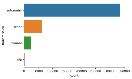
자동차의 트랜스미션 종류는 automatic이 가장 많다.
sns.countplot(y='drive', data=df.fillna('n/a'), order=df.fillna('n/a')['drive'].value_counts().index)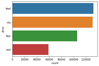
자동차의 구동 타입은 4wd가 가장 많다.
sns.countplot(y='size', data=df.fillna('n/a'), order=df.fillna('n/a')['size'].value_counts().index)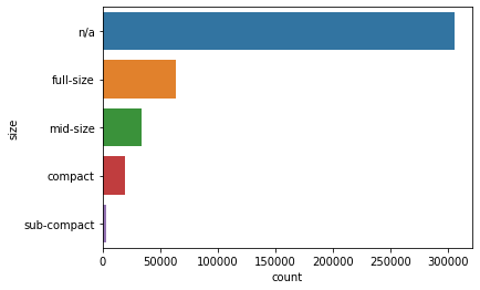
자동차 크기는 null 값이 가장 많고, 다음으로 full-size가 많다.
sns.countplot(y='type', data=df.fillna('n/a'), order=df.fillna('n/a')['type'].value_counts().index)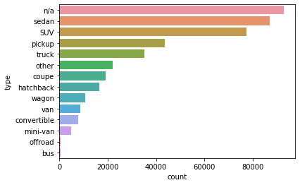
자동차의 일반 타입은 null 값이 가장 많고, 다음으로 sedan이 많다.
sns.countplot(y='paint_color', data=df.fillna('n/a'), order=df.fillna('n/a')['paint_color'].value_counts().index)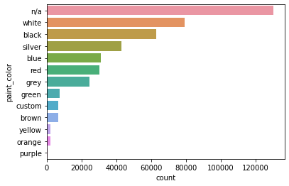
자동차 색상은 null 값이 가장 많고, 다음으로 white가 많다.
# seaborn의 rugplot()로 수치형 데이터 통계 그리기
# 값의 범위가 너무 넓을 경우 histplot()이 잘 동작하지 않음
fig = plt.figure(figsize=(8, 2))
sns.rugplot(x='price', data=df, height=1)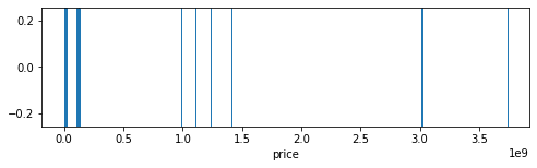
price 컬럼은 분석하기 힘들다.
fig = plt.figure(figsize=(8, 2))
sns.rugplot(x='odometer', data=df, height=1)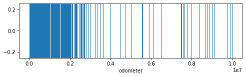
odometer 컬럼은 분석하기 힘들다.
# seaborn의 histplot()로 히스토그램 그리기
sns.histplot(x='age', data=df, bins=18, kde=True)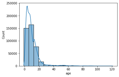
거래가 기입된 경과년도는 0 ~ 10년 사이가 가장 많다.
데이터 클리닝 수행
# seaborn의 boxplot()로 범주형 데이터 시각화
sns.boxplot(x='manufacturer', y='price', data=df.fillna('n/a'))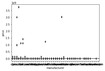
manufacturer 컬럼은 분석하기 힘들다.
sns.boxplot(x='fuel', y='price', data=df.fillna('n/a'))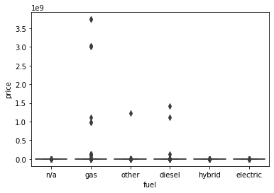
fuel 컬럼은 분석하기 힘들다.
# 범주형 데이터를 아래 방법 중 적절히 판단하여 처리
# 1. 결손 데이터가 포함된 Row 제거
# 2. 결손 데이터를 others 범주로 변경
# 3. 지나치게 소수로 이루어진 범주를 others 범주로 변경
# (4. Classifier를 학습해서 결손 데이터를 추정하여 채워넣기)
# 1. title_status
col = 'title_status'
counts = df[col].fillna('others').value_counts()
plt.grid()
plt.plot(range(len(counts)), counts)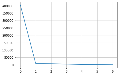
대부분 데이터가 같은 값을 가지므로 유용하지 않다. → 제거
df.drop('title_status', axis=1, inplace=True)
# 2. manufacturer
col = 'manufacturer'
counts = df[col].fillna('others').value_counts()
plt.grid()
plt.plot(range(len(counts)), counts)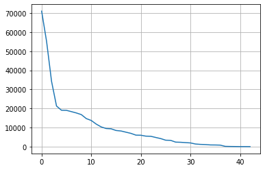
# 상위 10개의 값을 제외하고 모두 others 범주로 변경
n_categorical = 10
others = counts.index[n_categorical:]
df[col] = df[col].apply(lambda s: s if str(s) not in others else 'others')
df[col].value_counts()
others 139807
ford 70985
chevrolet 55064
toyota 34202
honda 21269
nissan 19067
jeep 19014
ram 18342
gmc 16785
bmw 14699
Name: manufacturer, dtype: int64
# 3. region
col = 'region'
counts = df[col].fillna('others').value_counts()
plt.grid()
plt.plot(range(len(counts)), counts)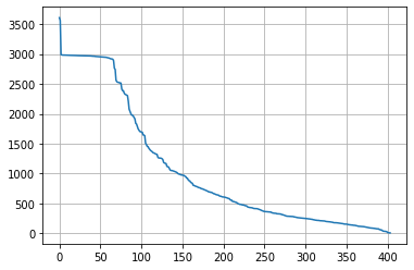
# 상위 5개의 값을 제외하고 모두 others 범주로 변경
n_categorical = 5
others = counts.index[n_categorical:]
df[col] = df[col].apply(lambda s: s if str(s) not in others else 'others')
df[col].value_counts()
others 410754
columbus 3608
jacksonville 3562
spokane / coeur d'alene 2988
eugene 2985
fresno / madera 2983
Name: region, dtype: int64
# 4. model
col = 'model'
counts = df[col].fillna('others').value_counts()
plt.grid()
plt.plot(range(len(counts[:20])), counts[:20])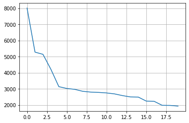
# 상위 10개의 값을 제외하고 모두 others 범주로 변경
n_categorical = 10
others = counts.index[n_categorical:]
df[col] = df[col].apply(lambda s: s if str(s) not in others else 'others')
df[col].value_counts()
others 386690
f-150 8009
silverado 1500 5140
1500 4211
camry 3135
silverado 3023
accord 2969
wrangler 2848
civic 2799
altima 2779
Name: model, dtype: int64
# 5. condition
col = 'condition'
counts = df[col].fillna('others').value_counts()
plt.grid()
plt.plot(range(len(counts)), counts)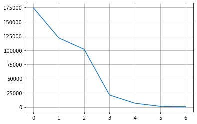
# 상위 3개의 값을 제외하고 모두 others 범주로 변경
n_categorical = 3
others = counts.index[n_categorical:]
df[col] = df[col].apply(lambda s: s if str(s) not in others else 'others')
df[col].value_counts()
good 121456
excellent 101467
others 29853
Name: condition, dtype: int64
# 6. cylinders
col = 'cylinders'
counts = df[col].fillna('others').value_counts()
plt.grid()
plt.plot(range(len(counts)), counts)
# 상위 4개의 값을 제외하고 모두 others 범주로 변경
n_categorical = 4
others = counts.index[n_categorical:]
df[col] = df[col].apply(lambda s: s if str(s) not in others else 'others')
df[col].value_counts()
6 cylinders 94169
4 cylinders 77642
8 cylinders 72062
others 5329
Name: cylinders, dtype: int64
# 7. fuel
col = 'fuel'
counts = df[col].fillna('others').value_counts()
plt.grid()
plt.plot(range(len(counts)), counts)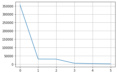
# 상위 2개의 값을 제외하고 모두 others 범주로 변경
n_categorical = 2
others = counts.index[n_categorical:]
df[col] = df[col].apply(lambda s: s if str(s) not in others else 'others')
df.loc[df[col] == 'other', col] = 'others'
df[col].value_counts()
gas 356209
others 67658
Name: fuel, dtype: int64
# 8. transmission
col = 'transmission'
counts = df[col].fillna('others').value_counts()
plt.grid()
plt.plot(range(len(counts)), counts)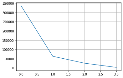
# 상위 3개의 값을 제외하고 모두 others 범주로 변경
n_categorical = 3
others = counts.index[n_categorical:]
df[col] = df[col].apply(lambda s: s if str(s) not in others else 'others')
df[col].value_counts()
automatic 336524
other 62682
manual 25118
Name: transmission, dtype: int64
# 9. drive
col = 'drive'
counts = df[col].fillna('others').value_counts()
plt.grid()
plt.plot(range(len(counts)), counts)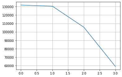
# 상위 3개의 값을 제외하고 모두 others 범주로 변경
n_categorical = 3
others = counts.index[n_categorical:]
df[col] = df[col].apply(lambda s: s if str(s) not in others else 'others')
df[col].fillna('others', inplace=True)
df[col].value_counts()
others 189459
4wd 131904
fwd 105517
Name: drive, dtype: int64
# 10. size
col = 'size'
counts = df[col].fillna('others').value_counts()
plt.grid()
plt.plot(range(len(counts)), counts)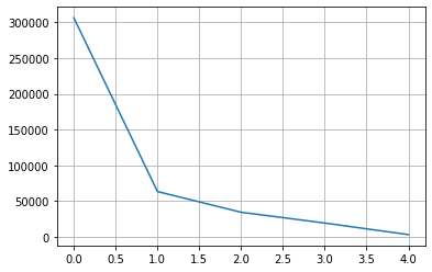
# 상위 2개의 값을 제외하고 모두 others 범주로 변경
n_categorical = 2
others = counts.index[n_categorical:]
df[col] = df[col].apply(lambda s: s if str(s) not in others else 'others')
df[col].value_counts()
full-size 63465
others 57054
Name: size, dtype: int64
# 11. type
col = 'type'
counts = df[col].fillna('others').value_counts()
plt.grid()
plt.plot(range(len(counts)), counts)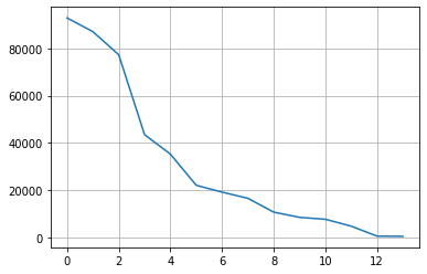
# 상위 8개의 값을 제외하고 모두 others 범주로 변경
n_categorical = 8
others = counts.index[n_categorical:]
df[col] = df[col].apply(lambda s: s if str(s) not in others else 'others')
df.loc[df[col] == 'other', col] = 'others'
df[col].value_counts()
sedan 87056
SUV 77284
others 55091
pickup 43510
truck 35279
coupe 19204
hatchback 16598
Name: type, dtype: int64
# 12. paint_color
col = 'paint_color'
counts = df[col].fillna('others').value_counts()
plt.grid()
plt.plot(range(len(counts)), counts)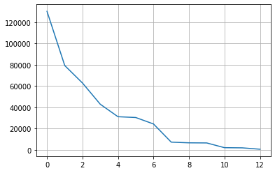
# 상위 7개의 값을 제외하고 모두 others 범주로 변경
n_categorical = 7
others = counts.index[n_categorical:]
df[col] = df[col].apply(lambda s: s if str(s) not in others else 'others')
df[col].value_counts()
white 79285
black 62861
silver 42970
blue 31223
red 30473
others 25449
grey 24416
Name: paint_color, dtype: int64
# 수치형 데이터 클리닝
# quantile()를 이용하여 outlier를 제거하고 시각화하여 확인
# quantile(0.99) = 상위 1% / quantile(0.1) = 하위 10%
p1 = df['price'].quantile(0.99)
p2 = df['price'].quantile(0.1)
print(p1, p2)  # 66995.0 500.0
df = df[(p1 > df['price']) & (df['price'] > p2)]
o1 = df['odometer'].quantile(0.99)
o2 = df['odometer'].quantile(0.1)
print(o1, o2)  # 280000.0 15812.0
df = df[(o1 > df['odometer']) & (df['odometer'] > o2)]
df.describe()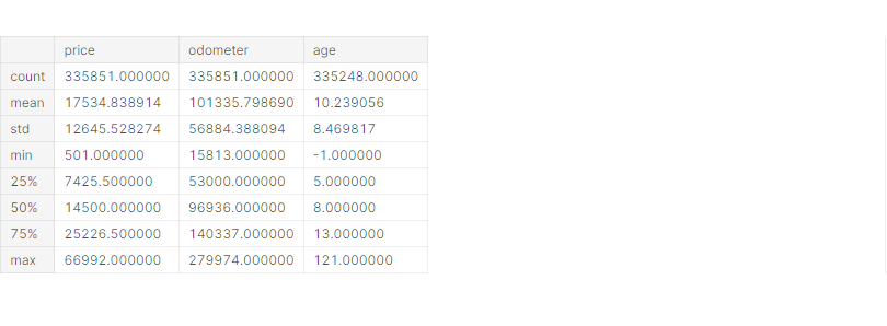
# seaborn의 boxplot()로 범주형 데이터 시각화
fig = plt.figure(figsize=(10, 5))
sns.boxplot(x='manufacturer', y='price', data=df)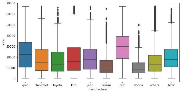
ram 에서 생산한 자동차의 가격이 대체적으로 높은 편이다.
fig = plt.figure(figsize=(14, 5))
sns.boxplot(x='model', y='price', data=df)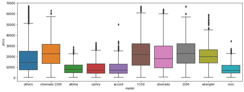
저가형 자동차와 고가형 자동차로 나뉘는 것을 알 수 있다.
# seaborn의 heatmap()로 correlation 시각화
# 절댓값으로 컬럼간의 상관관계 확인
sns.heatmap(df.corr(), annot=True, cmap='YlOrRd')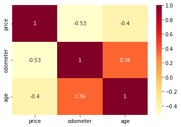
price(가격)는 age, odometer와 음의 상관관계를 가진다.
데이터 전처리
from sklearn.preprocessing import StandardScaler# StandardScaler을 이용하여 수치형 데이터 표준화
X_num = df[['odometer', 'age']]
scaler = StandardScaler()
scaler.fit(X_num)
X_scaled = scaler.transform(X_num)
X_scaled = pd.DataFrame(X_scaled, index=X_num.index, columns=X_num.columns)
# get_dummies를 이용하여 범주형 데이터를 one-hot 벡터로 변경
X_cat = df.drop(['price', 'odometer', 'age'], axis=1)
X_cat = pd.get_dummies(X_cat)
# 입출력 데이터 통합
X = pd.concat([X_scaled, X_cat], axis=1)
y = df['price']
X.isna().sum()
price 컬럼에는 아직 null 값이 존재한다.
X.fillna(0.0, inplace=True)학습 데이터와 테스트 데이터 분리
from sklearn.model_selection import train_test_split# train_test_split을 이용하여 학습 데이터와 테스트 데이터 분리
X_train, X_test, y_train, y_test = train_test_split(X, y, test_size=0.3, random_state=1)
Regression 모델 학습
1. XGBoost 모델
from xgboost import XGBRegressor# XGBRegressor 모델 생성/학습
model_reg = XGBRegressor()
model_reg.fit(X_train, y_train)
from sklearn.metrics import mean_absolute_error, mean_squared_error
from math import sqrt
# mean_absolute_error, rmse 결과 출력
pred = model_reg.predict(X_test)
print(mean_absolute_error(y_test, pred))
print(mean_squared_error(y_test, pred))MAE = 3766.257349829494
RMSE = 5601.781128058931
모델 학습 결과 심화 분석
1. 실제 값과 추측 값의 Scatter plot 시각화
plt.scatter(x=y_test, y=pred, alpha=0.005)
plt.plot([0, 60000], [0, 60000], 'r-')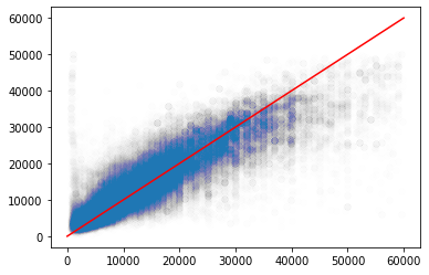
실제 값은 싼데 많이 비싼 것으로 오해하는 경우가 많다.
sns.histplot(x=y_test, y=pred)
plt.plot([0, 60000], [0, 60000], 'r-')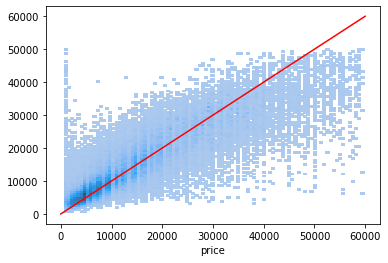
2. 에러 값의 히스토그램 확인
err = (pred - y_test) / y_test * 100
sns.histplot(err)
plt.xlabel('error (%)')
plt.xlim(-100, 100)
plt.grid()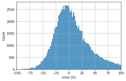
0 이하는 under estimate, 0 이상은 over estimate
err = pred - y_test
sns.histplot(err)
plt.xlabel('error ($)')
plt.grid()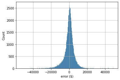
'데이터 분석 > 실습' 카테고리의 다른 글
| World Happiness Report up to 2020 (0) | 2022.01.05 |
|---|---|
| New York City Airbnb (0) | 2022.01.04 |
| US Election 2020 (0) | 2021.12.27 |
| European Soccer (0) | 2021.12.27 |
| League of Legends Diamond Ranked Games (10 min) (0) | 2021.12.23 |


