Video Game Sales with Ratings

데이터 분석/실습

Video Game Sales with Ratings

eunki 2022. 1. 6. 04:00

728x90

https://www.kaggle.com/rush4ratio/video-game-sales-with-ratings

Video Game Sales with Ratings

Video game sales from Vgchartz and corresponding ratings from Metacritic

www.kaggle.com

데이터 정보

Name: 게임의 이름
Platform: 게임이 동작하는 콘솔
Year_of_Release: 발매 년도
Genre: 게임의 장르
Publisher: 게임의 유통사
NA_Sales: 북미 판매량 (Millions)
EU_Sales: 유럽 연합 판매량 (Millions)
JP_Sales: 일본 판매량 (Millions)
Other_Sales: 기타 판매량 (아프리카, 일본 제외 아시아, 호주, EU 제외 유럽, 남미) (Millions)
Global_Sales: 전국 판매량
Critic_Score: Metacritic 스태프 점수
Critic_Count: Critic_Score에 사용된 점수의 수
User_Score: Metacritic 구독자의 점수
User_Count: User_Score에 사용된 점수의 수
Developer: 게임의 개발사
Rating: ESRB 등급 (19+, 17+ 등)

데이터셋 준비

import pandas as pd
import numpy as np
import matplotlib.pyplot as plt
import seaborn as sns

df = pd.read_csv('../input/video-game-sales-with-ratings/Video_Games_Sales_as_at_22_Dec_2016.csv')

EDA 및 데이터 기초 통계 분석

df.head()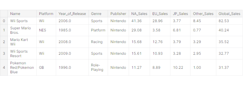

수치형 데이터: Year_of_Release, NA_Sales, EU_Sales, JP_Sales, Other_Sales, Critic_Score, Critic_Count, User_Score, User_Count
범주형 데이터: Name, Platform, Genre, Publisher, Developer, Rating
타겟 데이터: Global_Sales

df.info()

<class 'pandas.core.frame.DataFrame'>
RangeIndex: 16719 entries, 0 to 16718
Data columns (total 16 columns):
 #   Column           Non-Null Count  Dtype  
---  ------           --------------  -----  
 0   Name             16717 non-null  object 
 1   Platform         16719 non-null  object 
 2   Year_of_Release  16450 non-null  float64
 3   Genre            16717 non-null  object 
 4   Publisher        16665 non-null  object 
 5   NA_Sales         16719 non-null  float64
 6   EU_Sales         16719 non-null  float64
 7   JP_Sales         16719 non-null  float64
 8   Other_Sales      16719 non-null  float64
 9   Global_Sales     16719 non-null  float64
 10  Critic_Score     8137 non-null   float64
 11  Critic_Count     8137 non-null   float64
 12  User_Score       10015 non-null  object 
 13  User_Count       7590 non-null   float64
 14  Developer        10096 non-null  object 
 15  Rating           9950 non-null   object 
dtypes: float64(9), object(7)
memory usage: 2.0+ MB

(16719, 16) → 16719 rows 16 columns

df.isna().sum()

Name                  2
Platform              0
Year_of_Release     269
Genre                 2
Publisher            54
NA_Sales              0
EU_Sales              0
JP_Sales              0
Other_Sales           0
Global_Sales          0
Critic_Score       8582
Critic_Count       8582
User_Score         6704
User_Count         9129
Developer          6623
Rating             6769
dtype: int64

null 값이 존재하는 컬럼들이 있다. → 제거

# 결손 데이터가 포함된 row 제거
df.dropna(inplace=True)

df.head()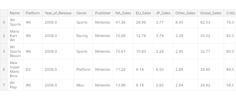

# User_Score 컬럼 값은 object이므로 float으로 형변환
df['User_Score'] = df['User_Score'].apply(float)

# seaborn의 histplot()로 히스토그램 그리기
sns.histplot(x='Year_of_Release', data=df, bins=16)

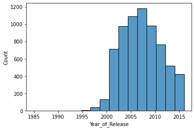
게임 발매 년도는 2005 ~ 2010년이 가장 많다.

sns.histplot(x='Global_Sales', data=df)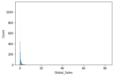

outlier로 인해 값의 범위가 넓어서 분석하기 어렵다.

sns.rugplot(x='Global_Sales', data=df)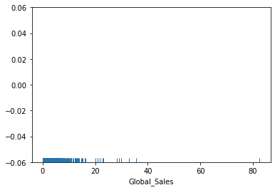

df[df['Global_Sales'] > 30]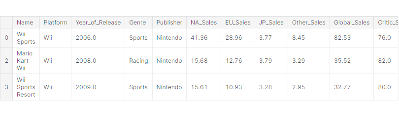

# 전국 판매량의 상위 1%
gs = df['Global_Sales'].quantile(0.99)
gs  # 7.167600000000002

df = df[df['Global_Sales'] < gs]

전국 판매량의 상위 1% 값은 제거한다.

sns.histplot(x='Global_Sales', data=df)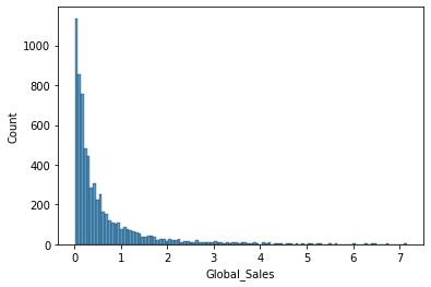

대부분 게임들의 전국 판매량은 낮은 편이다.

fig = plt.figure(figsize=(20, 5))
sns.histplot(x='Global_Sales', hue='Genre', data=df, kde=True)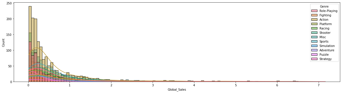

sns.histplot(x='Critic_Score', data=df, bins=16)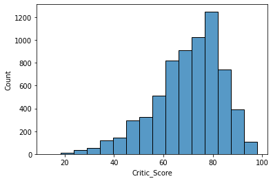

Metacritic 스태프 점수는 80점이 가장 많다.

sns.histplot(x='User_Score', data=df, bins=16)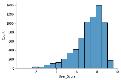

Metacritic 구독자 점수는 8점이 가장 많다.

sns.histplot(x='Critic_Count', data=df, bins=16)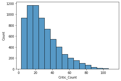

Critic_Score에 사용된 점수의 수는 10 ~ 20개가 가장 많다.

sns.histplot(x='User_Count', data=df)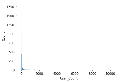

outlier로 인해 값의 범위가 넓어서 분석하기 어렵다.

sns.rugplot(x='User_Count', data=df)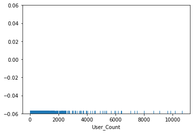

# User_Score에 사용된 점수의 수의 상위 3%
uc = df['User_Count'].quantile(0.97)
uc  # 1165.4499999999962

df = df[df['User_Count'] < uc]

User_Score에 사용된 점수의 수의 상위 3% 값은 제거한다.

sns.histplot(x='User_Count', data=df)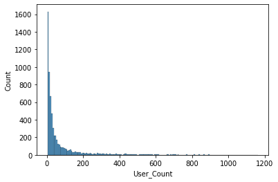

대부분 게임들의 User_Score에 사용된 점수의 수는 낮은 편이다

# seaborn의 jointplot()로 산점도와 히스토그램을 함께 그리기
sns.jointplot(x='Year_of_Release', y='Global_Sales', data=df, kind='hist')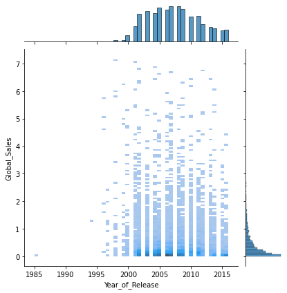

게임 발매 년도와 전국 판매량은 거의 상관관계가 없다.

sns.jointplot(x='Critic_Score', y='Global_Sales', data=df, kind='hist')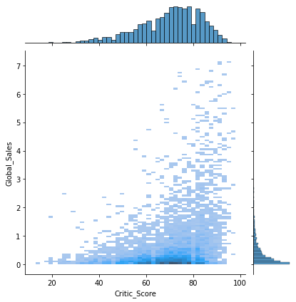

Critic_Score가 전국 판매량을 완전히 보장하지는 않지만, Critic_Score가 낮은 게임들은 높은 판매량을 가지지 않는다.

sns.jointplot(x='User_Score', y='Global_Sales', data=df, kind='hist')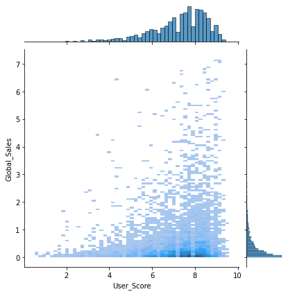

User_Score는 판매가 이루어진 이후에 생긴 값이기 때문에 학습에서 제외한다.

sns.jointplot(x='Critic_Count', y='Global_Sales', data=df, kind='hist')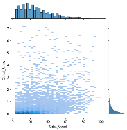

Critic_Count가 많다는 것은 기대작이라는 것을 의미한다.
Critic_Count가 많을수록 게임 판매량도 많은 것으로 보인다.

sns.jointplot(x='User_Count', y='Global_Sales', data=df, kind='hist')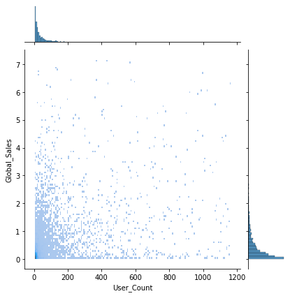

User_Count는 판매가 이루어진 이후에 생긴 값이기 때문에 학습에서 제외한다.

# 범주형 데이터별 전국 판매량의 Boxplot 시각화
fig = plt.figure(figsize=(15, 5))
sns.boxplot(x='Platform', y='Global_Sales', data=df)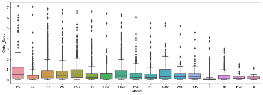

플레이스테이션(PS)의 전국 게임 판매량이 가장 높은 편이다.
컴퓨터(PC)의 전국 게임 판매량은 가장 낮은 편이지만, 게임이 워낙 많고 다양해서 낮은 것으로 예상된다.

fig = plt.figure(figsize=(15, 5))
sns.boxplot(x='Genre', y='Global_Sales', data=df)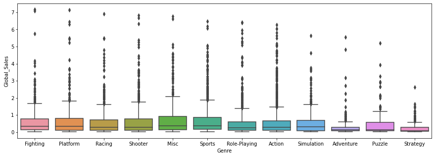

Misc와 Sports 장르의 게임이 전국 판매량이 높은 편이다.
Adventure 장르의 게임은 전국 판매량이 낮은 편이다.

fig = plt.figure(figsize=(15, 5))
sns.boxplot(x='Publisher', y='Global_Sales', data=df)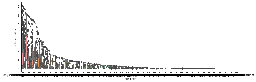

게임의 유통사가 너무 많아서 분석하기 힘들다.

fig = plt.figure(figsize=(15, 5))
sns.boxplot(x='Developer', y='Global_Sales', data=df)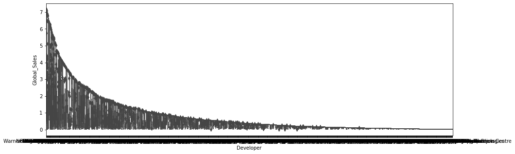

게임의 개발사가 너무 많아서 분석하기 힘들다.

# 전문가 평점과 사용자 평점의 통계 비교/분석
sns.boxplot(y='Critic_Score', data=df)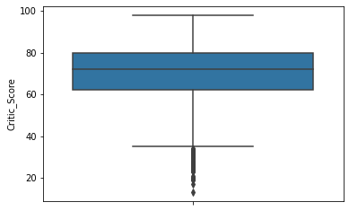

sns.boxplot(y='User_Score', data=df)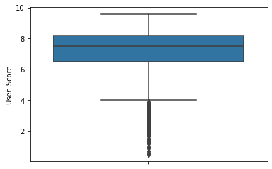

전문가 평점과 사용자 평점 값의 범위가 다르므로 동일하게 맞추어서 비교한다.

critic_score = df[['Critic_Score']].copy()
critic_score.rename({'Critic_Score': 'Score'}, axis=1, inplace=True)
critic_score['ScoreBy'] = 'Critics'
critic_score

user_score = df[['User_Score']].copy() * 10
user_score.rename({'User_Score': 'Score'}, axis=1, inplace=True)
user_score['ScoreBy'] = 'Users'
user_score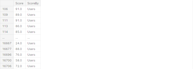

scores = pd.concat([critic_score, user_score])
scores

sns.boxplot(x='ScoreBy', y='Score', data=scores)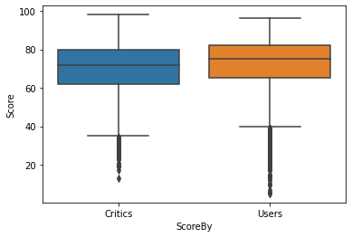

사용자 평점이 전문가 평점보다 조금 높은 편이지만 거의 비슷하다.

sns.boxplot(x='Genre', y='Critic_Score', data=df)
plt.xticks(rotation=90)
plt.show()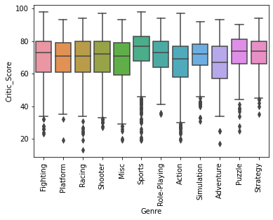

Sports 장르의 게임이 Metacritic 스태프 점수가 높은 편이다.

sns.boxplot(x='Genre', y='Critic_Count', data=df)
plt.xticks(rotation=90)
plt.show()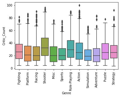

Shooter와 Role-Playing 장르의 게임이 Critic_Score에 사용된 점수의 수가 많은 편이다.

sns.boxplot(x='Genre', y='User_Score', data=df)
plt.xticks(rotation=90)
plt.show()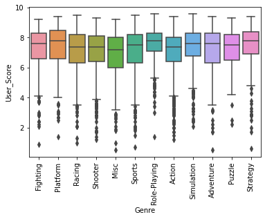

Role-Playing 장르의 게임이 Metacritic 구독자의 점수가 높은 편이다.

# 수치형 데이터간의 상관성 시각화
fig = plt.figure(figsize=(8, 8))
sns.heatmap(df.corr(), annot=True, cmap='YlOrRd')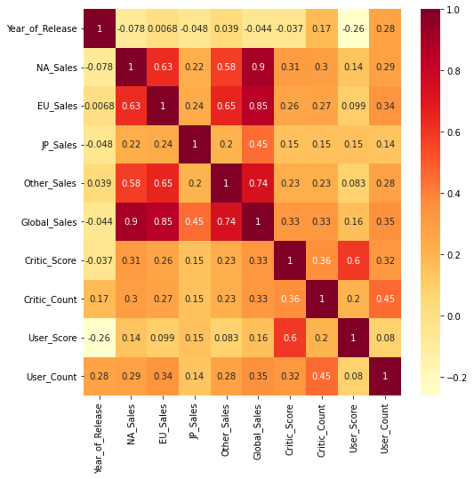

판매량(Global_Sales)이 높다고 해서 User_Score가 높은 것은 아니다.
발매 년도(Year_of_Release)가 최근일수록 User_Score가 낮다.

데이터 클리닝 수행

# 범주형 데이터에서 소수 범주를 others로 대체
pb = df['Publisher'].value_counts()
plt.plot(range(len(pb)), pb)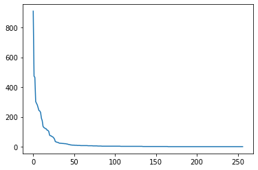

# 상위 20개의 값을 제외하고 모두 others 범주로 변경
df['Publisher'] = df['Publisher'].apply(lambda s: s if s not in pb[20:] else 'others')

fig = plt.figure(figsize=(15, 6))
sns.countplot(x='Publisher', data=df)
plt.xticks(rotation=90)
plt.show()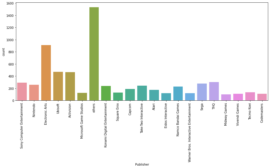

게임의 유통사(Publisher)는 others가 가장 많고, 다음으로 Electronic Arts(EA)가 많다.

fig = plt.figure(figsize=(15, 6))
sns.boxplot(x='Publisher', y='Global_Sales', data=df)
plt.xticks(rotation=90)
plt.show()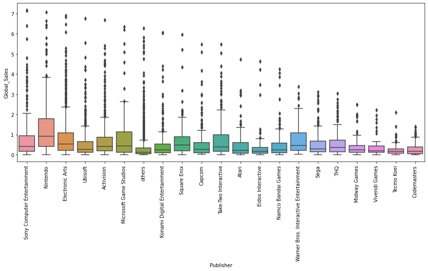

Nintendo 유통사의 전국 판매량이 가장 높은 편이다.

pb = df['Developer'].value_counts()
plt.plot(range(len(pb)), pb)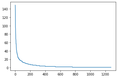

# 상위 20개의 값을 제외하고 모두 others 범주로 변경
df['Developer'] = df['Developer'].apply(lambda s: s if s not in pb[20:] else 'others')

fig = plt.figure(figsize=(15, 6))
sns.boxplot(x='Developer', y='Global_Sales', data=df)
plt.xticks(rotation=90)
plt.show()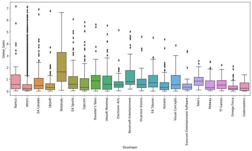

Nintendo 개발사의 전국 판매량이 가장 높은 편이다.

데이터 전처리

# get_dummies를 이용하여 범주형 데이터를 one-hot 벡터로 변경
X_cat = df[['Platform', 'Genre', 'Publisher']]
X_cat = pd.get_dummies(X_cat, drop_first=True)

from sklearn.preprocessing import StandardScaler

# StandardScaler을 이용하여 수치형 데이터 표준화
X_num = df[['Year_of_Release', 'Critic_Score', 'Critic_Count']]

scaler = StandardScaler()
scaler.fit(X_num)
X_scaled = scaler.transform(X_num)
X_scaled = pd.DataFrame(X_scaled, index=X_num.index, columns=X_num.columns)

X = pd.concat([X_cat, X_scaled], axis=1)
y = df['Global_Sales']

X.head()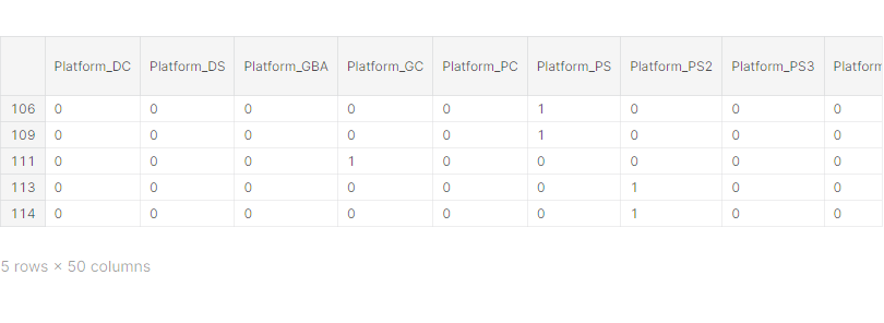

학습 데이터와 테스트 데이터 분리

from sklearn.model_selection import train_test_split

# train_test_split을 이용하여 학습 데이터와 테스트 데이터 분리
X_train, X_test, y_train, y_test = train_test_split(X, y, test_size=0.3, random_state=1)

Regression 모델 학습

1. XGBoost 모델

from xgboost import XGBRegressor

# XGBRegressor 모델 생성/학습
model_xgb = XGBRegressor()
model_xgb.fit(X_train, y_train)

XGBRegressor(base_score=0.5, booster='gbtree', colsample_bylevel=1,
             colsample_bynode=1, colsample_bytree=1, enable_categorical=False,
             gamma=0, gpu_id=-1, importance_type=None,
             interaction_constraints='', learning_rate=0.300000012,
             max_delta_step=0, max_depth=6, min_child_weight=1, missing=nan,
             monotone_constraints='()', n_estimators=100, n_jobs=4,
             num_parallel_tree=1, predictor='auto', random_state=0, reg_alpha=0,
             reg_lambda=1, scale_pos_weight=1, subsample=1, tree_method='exact',
             validate_parameters=1, verbosity=None)

2. Linear Regression 모델

from sklearn.linear_model import LinearRegression

# LinearRegression 모델 생성/학습
model_lr = LinearRegression()
model_lr.fit(X_train, y_train)

from sklearn.metrics import mean_absolute_error, mean_squared_error
from math import sqrt

# mean_absolute_error, rmse 결과 출력
pred_xgb = model_xgb.predict(X_test)
pred_lr = model_lr.predict(X_test)

print('XGB MAE: ', mean_absolute_error(y_test, pred_xgb))
print('XGB RMSE: ', sqrt(mean_squared_error(y_test, pred_xgb)))

print('LR MAE: ', mean_absolute_error(y_test, pred_lr))
print('LR RMSE: ', sqrt(mean_squared_error(y_test, pred_lr)))

XGB MAE:  0.4028702780745956
XGB RMSE:  0.6961683526556979
LR MAE:  0.4567498509022437
LR RMSE:  0.7196767623667085

모델 학습 결과 심화 분석

1. 실제 값과 추측 값의 Scatter plot 시각화

plt.scatter(y_test, pred_xgb, alpha=0.1)
plt.plot([0, 8], [0, 8], 'r-')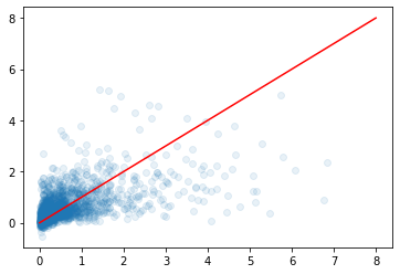

under_estimate 경향이 있다.
판매량이 많은 게임의 데이터가 거의 없어서 에러가 많이 난다.

plt.scatter(y_test, pred_lr, alpha=0.1)
plt.plot([0, 8], [0, 8], 'r-')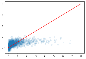

2. XGBoost 모델로 특징의 중요도 확인

fig = plt.figure(figsize=(15, 5))
plt.bar(X.columns, model_xgb.feature_importances_)
plt.xticks(rotation=90)
plt.show()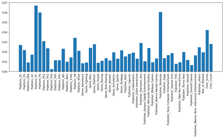

Platform_PC 피쳐 중요도가 가장 높다.

유저 평점 Regression 모델 학습

# StandardScaler을 이용하여 수치형 데이터 표준화
X_num = df[['Year_of_Release', 'Critic_Score', 'Critic_Count']]

scaler = StandardScaler()
scaler.fit(X_num)
X_scaled = scaler.transform(X_num)
X_scaled = pd.DataFrame(X_scaled, index=X_num.index, columns=X_num.columns)

X = pd.concat([X_cat, X_scaled], axis=1)
y = df['User_Score']

# train_test_split을 이용하여 학습 데이터와 테스트 데이터 분리
X_train, X_test, y_train, y_test = train_test_split(X, y, test_size=0.3, random_state=1)

# XGBRegressor 모델 생성/학습
model_xgb = XGBRegressor()
model_xgb.fit(X_train, y_train)

XGBRegressor(base_score=0.5, booster='gbtree', colsample_bylevel=1,
             colsample_bynode=1, colsample_bytree=1, enable_categorical=False,
             gamma=0, gpu_id=-1, importance_type=None,
             interaction_constraints='', learning_rate=0.300000012,
             max_delta_step=0, max_depth=6, min_child_weight=1, missing=nan,
             monotone_constraints='()', n_estimators=100, n_jobs=4,
             num_parallel_tree=1, predictor='auto', random_state=0, reg_alpha=0,
             reg_lambda=1, scale_pos_weight=1, subsample=1, tree_method='exact',
             validate_parameters=1, verbosity=None)

# LinearRegression 모델 생성/학습
model_lr = LinearRegression()
model_lr.fit(X_train, y_train)

# mean_absolute_error, rmse 결과 출력
pred_xgb = model_xgb.predict(X_test)
pred_lr = model_lr.predict(X_test)

print('XGB MAE: ', mean_absolute_error(y_test, pred_xgb))
print('XGB RMSE: ', sqrt(mean_squared_error(y_test, pred_xgb)))

print('LR MAE: ', mean_absolute_error(y_test, pred_lr))
print('LR RMSE: ', sqrt(mean_squared_error(y_test, pred_lr)))

XGB MAE:  0.7737539779133376
XGB RMSE:  1.0453455989321712
LR MAE:  0.7705374527545784
LR RMSE:  1.0304538778673875

plt.scatter(y_test, pred_xgb, alpha=0.1)
plt.plot([0, 10], [0, 10], 'r-')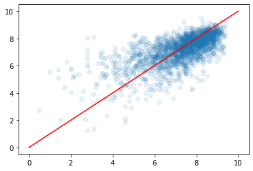

plt.scatter(y_test, pred_lr, alpha=0.1)
plt.plot([0, 10], [0, 10], 'r-')

fig = plt.figure(figsize=(15, 5))
plt.bar(X.columns, model_xgb.feature_importances_)
plt.xticks(rotation=90)
plt.show()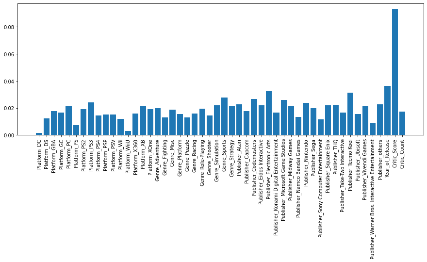

Critic_Score 피쳐 중요도가 가장 높다.

728x90