World Happiness Report up to 2020

데이터 분석/실습

World Happiness Report up to 2020

eunki 2022. 1. 5. 22:08

728x90

https://www.kaggle.com/mathurinache/world-happiness-report

World Happiness Report up to 2020

Bliss scored agreeing to financial, social, etc.

www.kaggle.com

데이터 정보

Country: 국가
Region: 국가의 지역
Happiness Rank: 행복지수 순위
Happiness Score: 행복지수 점수
GDP per capita: 1인당 GDP
Healthy Life Expectancy: 건강 기대수명
Social support: 사회적 지원
Freedom to make life choices: 삶에 대한 선택의 자유
Generosity: 관용
Corruption Perception: 부정부패
Dystopia + Residual: 그 외

데이터셋 준비

import pandas as pd
import numpy as np
import matplotlib.pyplot as plt
import seaborn as sns

df = dict()
df['2015'] = pd.read_csv('../input/world-happiness-report/2015.csv')
df['2016'] = pd.read_csv('../input/world-happiness-report/2016.csv')
df['2017'] = pd.read_csv('../input/world-happiness-report/2017.csv')
df['2018'] = pd.read_csv('../input/world-happiness-report/2018.csv')
df['2019'] = pd.read_csv('../input/world-happiness-report/2019.csv')
df['2020'] = pd.read_csv('../input/world-happiness-report/2020.csv')

데이터프레임 구성

# 각 데이터 프레임의 컬럼 확인
for key in df:
    print(key, df[key].columns)

2015 Index(['Country', 'Region', 'Happiness Rank', 'Happiness Score',
       'Standard Error', 'Economy (GDP per Capita)', 'Family',
       'Health (Life Expectancy)', 'Freedom', 'Trust (Government Corruption)',
       'Generosity', 'Dystopia Residual'],
      dtype='object')
2016 Index(['Country', 'Region', 'Happiness Rank', 'Happiness Score',
       'Lower Confidence Interval', 'Upper Confidence Interval',
       'Economy (GDP per Capita)', 'Family', 'Health (Life Expectancy)',
       'Freedom', 'Trust (Government Corruption)', 'Generosity',
       'Dystopia Residual'],
      dtype='object')
2017 Index(['Country', 'Happiness.Rank', 'Happiness.Score', 'Whisker.high',
       'Whisker.low', 'Economy..GDP.per.Capita.', 'Family',
       'Health..Life.Expectancy.', 'Freedom', 'Generosity',
       'Trust..Government.Corruption.', 'Dystopia.Residual'],
      dtype='object')
2018 Index(['Overall rank', 'Country or region', 'Score', 'GDP per capita',
       'Social support', 'Healthy life expectancy',
       'Freedom to make life choices', 'Generosity',
       'Perceptions of corruption'],
      dtype='object')
2019 Index(['Overall rank', 'Country or region', 'Score', 'GDP per capita',
       'Social support', 'Healthy life expectancy',
       'Freedom to make life choices', 'Generosity',
       'Perceptions of corruption'],
      dtype='object')
2020 Index(['Country name', 'Regional indicator', 'Ladder score',
       'Standard error of ladder score', 'upperwhisker', 'lowerwhisker',
       'Logged GDP per capita', 'Social support', 'Healthy life expectancy',
       'Freedom to make life choices', 'Generosity',
       'Perceptions of corruption', 'Ladder score in Dystopia',
       'Explained by: Log GDP per capita', 'Explained by: Social support',
       'Explained by: Healthy life expectancy',
       'Explained by: Freedom to make life choices',
       'Explained by: Generosity', 'Explained by: Perceptions of corruption',
       'Dystopia + residual'],
      dtype='object')

각 데이터 프레임은 서로 다른 column 구성을 가지고 있다.

# 각 년도별로 다른 정보를 가진 데이터 프레임의 Column을 동일하게 표준화
cols = ['country', 'score', 'economy', 'family', 'health', 'freedom', 'generosity', 'trust', 'residual']

df['2015'].drop(['Region', 'Happiness Rank', 'Standard Error'], axis=1, inplace=True)  # generosity, trust 순서 반대
df['2016'].drop(['Region', 'Happiness Rank', 
                 'Lower Confidence Interval', 'Upper Confidence Interval'], axis=1, inplace=True)  # generosity, trust 순서 반대
df['2017'].drop(['Happiness.Rank', 'Whisker.high', 'Whisker.low'], axis=1, inplace=True)
df['2018'].drop(['Overall rank'], axis=1, inplace=True)  # residual 없음
df['2019'].drop(['Overall rank'], axis=1, inplace=True)  # residual 없음
df['2020'].drop(['Regional indicator', 'Standard error of ladder score', 
                 'upperwhisker', 'lowerwhisker', 'Logged GDP per capita', 
                 'Social support', 'Healthy life expectancy', 
                 'Freedom to make life choices', 'Generosity',
                 'Perceptions of corruption', 'Ladder score in Dystopia',], axis=1, inplace=True)

# axis=0 : 각 column별 합계
# axis=1 : 각 record별 합계
df['2018'][['GDP per capita', 'Social support', 'Healthy life expectancy',
            'Freedom to make life choices', 'Generosity', 'Perceptions of corruption']].sum(axis=1)

0      5.047
1      5.211
2      5.184
3      5.069
4      5.169
       ...  
151    2.249
152    2.675
153    1.564
154    0.595
155    1.153
Length: 156, dtype: float64

# residual 컬럼 생성
df['2018']['residual'] = df['2018']['Score'] - df['2018'][['GDP per capita', 'Social support', 'Healthy life expectancy',
            'Freedom to make life choices', 'Generosity', 'Perceptions of corruption']].sum(axis=1)
df['2019']['residual'] = df['2019']['Score'] - df['2019'][['GDP per capita', 'Social support', 'Healthy life expectancy',
            'Freedom to make life choices', 'Generosity', 'Perceptions of corruption']].sum(axis=1)

df['2018'].head()

df['2015'].columns

Index(['Country', 'Happiness Score', 'Economy (GDP per Capita)', 'Family',
       'Health (Life Expectancy)', 'Freedom', 'Trust (Government Corruption)',
       'Generosity', 'Dystopia Residual'],
      dtype='object')

# generosity, trust 컬럼 순서 변경
df['2015'] = df['2015'][['Country', 'Happiness Score', 'Economy (GDP per Capita)', 'Family',
       'Health (Life Expectancy)', 'Freedom', 'Generosity', 'Trust (Government Corruption)',
       'Dystopia Residual']]
df['2016'] = df['2016'][['Country', 'Happiness Score', 'Economy (GDP per Capita)', 'Family',
       'Health (Life Expectancy)', 'Freedom', 'Generosity', 'Trust (Government Corruption)',
       'Dystopia Residual']]

# 각 데이터 프레임의 컬럼 다시 확인
for key in df:
    print(key, df[key].columns)

2015 Index(['Country', 'Happiness Score', 'Economy (GDP per Capita)', 'Family',
       'Health (Life Expectancy)', 'Freedom', 'Generosity',
       'Trust (Government Corruption)', 'Dystopia Residual'],
      dtype='object')
2016 Index(['Country', 'Happiness Score', 'Economy (GDP per Capita)', 'Family',
       'Health (Life Expectancy)', 'Freedom', 'Generosity',
       'Trust (Government Corruption)', 'Dystopia Residual'],
      dtype='object')
2017 Index(['Country', 'Happiness.Score', 'Economy..GDP.per.Capita.', 'Family',
       'Health..Life.Expectancy.', 'Freedom', 'Generosity',
       'Trust..Government.Corruption.', 'Dystopia.Residual'],
      dtype='object')
2018 Index(['Country or region', 'Score', 'GDP per capita', 'Social support',
       'Healthy life expectancy', 'Freedom to make life choices', 'Generosity',
       'Perceptions of corruption', 'residual'],
      dtype='object')
2019 Index(['Country or region', 'Score', 'GDP per capita', 'Social support',
       'Healthy life expectancy', 'Freedom to make life choices', 'Generosity',
       'Perceptions of corruption', 'residual'],
      dtype='object')
2020 Index(['Country name', 'Ladder score', 'Explained by: Log GDP per capita',
       'Explained by: Social support', 'Explained by: Healthy life expectancy',
       'Explained by: Freedom to make life choices',
       'Explained by: Generosity', 'Explained by: Perceptions of corruption',
       'Dystopia + residual'],
      dtype='object')

# 각 데이터 프레임의 컬럼 이름 통일
for col_name in df:
    df[col_name].columns = cols

# 각 데이터 프레임의 컬럼 다시 확인
for key in df:
    print(key, df[key].columns)

2015 Index(['country', 'score', 'economy', 'family', 'health', 'freedom',
       'generosity', 'trust', 'residual'],
      dtype='object')
2016 Index(['country', 'score', 'economy', 'family', 'health', 'freedom',
       'generosity', 'trust', 'residual'],
      dtype='object')
2017 Index(['country', 'score', 'economy', 'family', 'health', 'freedom',
       'generosity', 'trust', 'residual'],
      dtype='object')
2018 Index(['country', 'score', 'economy', 'family', 'health', 'freedom',
       'generosity', 'trust', 'residual'],
      dtype='object')
2019 Index(['country', 'score', 'economy', 'family', 'health', 'freedom',
       'generosity', 'trust', 'residual'],
      dtype='object')
2020 Index(['country', 'score', 'economy', 'family', 'health', 'freedom',
       'generosity', 'trust', 'residual'],
      dtype='object')

모든 데이터 프레임의 컬럼 구성이 동일해졌다.

# 하나의 데이터 프레임으로 결합
df_all = pd.concat(df)
df_all.index.names = ['year', 'rank']
df_all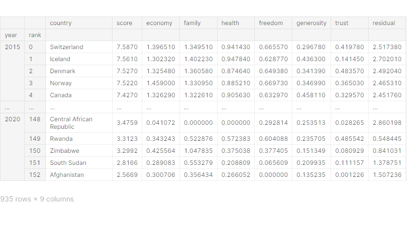

# 원하는 형태로 데이터 프레임 변형
df_all.reset_index(inplace=True)
df_all['rank'] += 1
df_all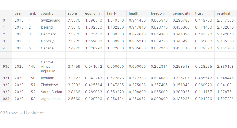

# pivot()을 이용하여 데이터 프레임 재구성
rank_table = df_all.pivot(index='country', columns='year', values='rank')
rank_table.sort_values('2020', inplace=True)
rank_table.head(20)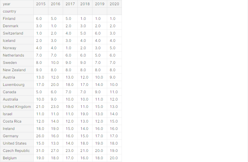

데이터 시각화

# 년도별 순위 변화 시각화
fig = plt.figure(figsize=(10, 50))
rank2020 = rank_table['2020'].dropna()
for c in rank2020.index:
    t = rank_table.loc[c].dropna()
    plt.plot(t.index, t, '.-')

plt.xlim(['2015', '2020'])  # x축 범위 제한
plt.ylim([0, rank_table.max().max() + 1])  # y축 범위 제한
plt.yticks(rank2020, rank2020.index)  # y축 눈금 표시(위치, 값)
ax = plt.gca()
ax.invert_yaxis()  # y축 반전
ax.yaxis.set_label_position('right')  # y축 눈금 오른쪽에 표시
ax.yaxis.tick_right()  # y축 눈금 오른쪽에 표시
plt.tight_layout()  # subplot간의 간격 조절
plt.show()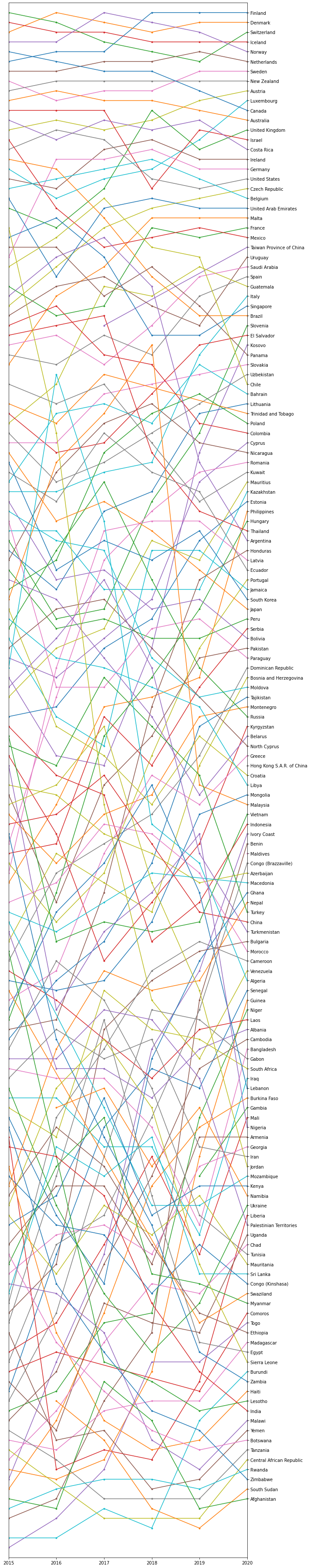

# 분야별로 나누어 점수 시각화
data = df_all[df_all['year'] == '2020']
data = data.loc[data.index[:20]]  # 행복지수 상위 20개 국가

d = data[data.columns[4:]].cumsum(axis=1)  # record간 누적합 적용
d = d[d.columns[::-1]]  # columns 순서 반대로 변경
d['country'] = data['country']  # country 컬럼 추가
d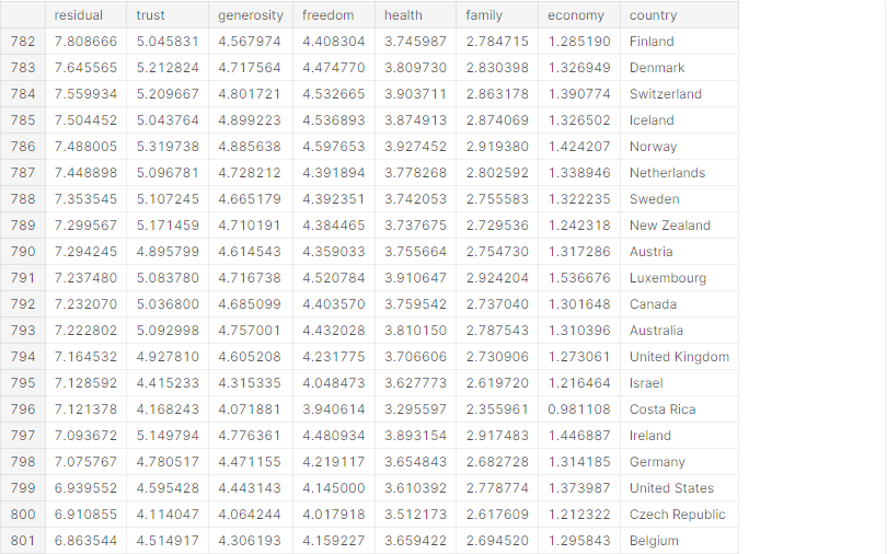

fig = plt.figure(figsize=(6, 8))

# 색을 정의하지 않으면 같은 색으로 칠해짐
sns.set_color_codes('muted')  # 톤다운
colors = ['r', 'g', 'b', 'c', 'm', 'y', 'purple'][::-1]
for idx, c in enumerate(d.columns[:-1]):
    sns.barplot(x=c, y='country', data=d, label=c, color=colors[idx])
    
plt.legend()
plt.title('Top 20 Happiness Scores in Details')
plt.xlabel('Happiness Score')
sns.despine(left=True, bottom=True)  # 프레임 제거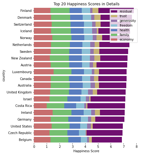

# column간의 상관성 시각화
sns.heatmap(df_all.drop('rank', axis=1).corr(), annot=True, cmap='YlOrRd')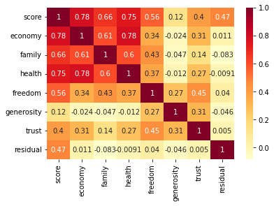

residual은 다른 변수들과 상관성이 거의 없어서 예측하기 힘들다.

sns.pairplot(df_all.drop('rank', axis=1))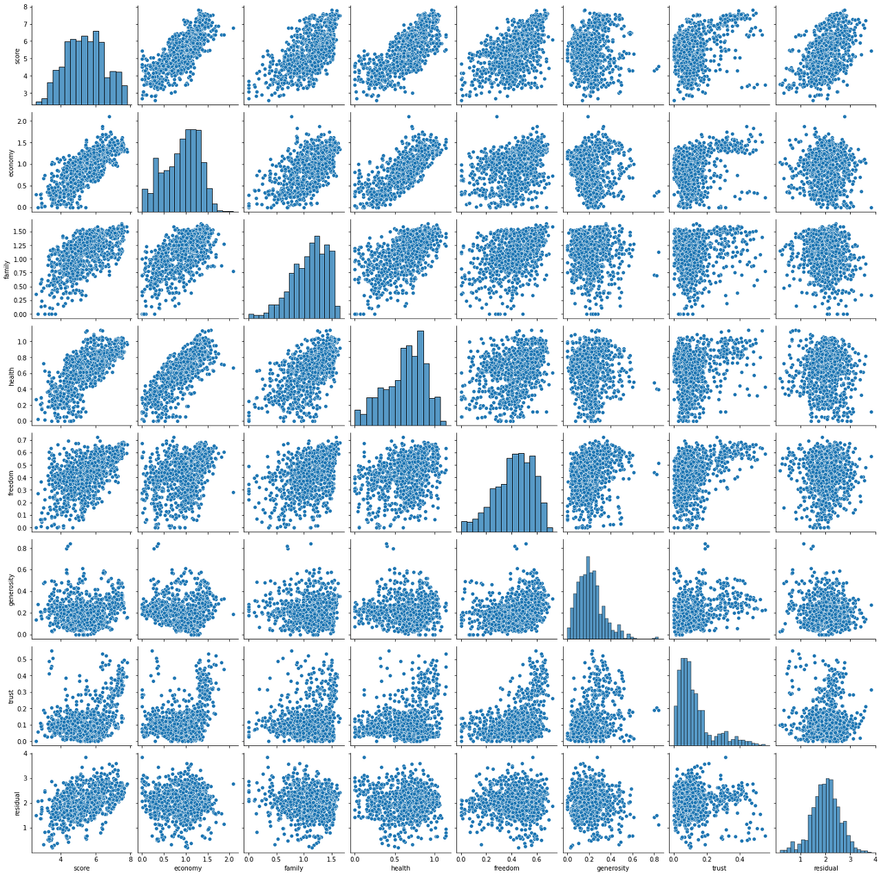

데이터 전처리

# 학습할 모델의 입출력 정의
col_input_list = ['economy', 'family', 'health', 'freedom', 'generosity', 'trust']
col_out = 'score'

# 학습 데이터와 테스트 데이터 분리
# 2015년 ~ 2019년도 데이터를 학습 데이터로, 2020년도 데이터를 테스트 데이터로 분리
df_train = df_all[df_all['year'] != '2020']
df_test = df_all[df_all['year'] == '2020']

X_train = df_train[col_input_list]
y_train= df_train[col_out]
X_test = df_test[col_input_list]
y_test= df_test[col_out]

from sklearn.preprocessing import StandardScaler

# StandardScaler을 이용하여 수치형 데이터 표준화
scaler = StandardScaler()
scaler.fit(X_train)

X_norm = scaler.transform(X_train)
X_train = pd.DataFrame(X_norm, index=X_train.index, columns=X_train.columns)

X_norm = scaler.transform(X_test)
X_test = pd.DataFrame(X_norm, index=X_test.index, columns=X_test.columns)

Regression 모델 학습

1. Linear Regression 모델

from sklearn.linear_model import LinearRegression

X_train.fillna(0, inplace=True)

# LinearRegression 모델 생성/학습
model_lr = LinearRegression()
model_lr.fit(X_train, y_train)

from sklearn.metrics import mean_absolute_error, mean_squared_error
from math import sqrt

# mean_absolute_error, rmse 결과 출력
pred = model_lr.predict(X_test)
print(mean_absolute_error(y_test, pred))  # 0.4411766043832983
print(mean_squared_error(y_test, pred))  # 0.32112983282430896

MAE = 0.4411766043832983
RMSE = 0.32112983282430896

2. XGBoost Regression 모델

from xgboost import XGBRegressor

# XGBRegressor 모델 생성/학습
model_xgb = XGBRegressor()
model_xgb.fit(X_train, y_train)

XGBRegressor(base_score=0.5, booster='gbtree', colsample_bylevel=1,
             colsample_bynode=1, colsample_bytree=1, enable_categorical=False,
             gamma=0, gpu_id=-1, importance_type=None,
             interaction_constraints='', learning_rate=0.300000012,
             max_delta_step=0, max_depth=6, min_child_weight=1, missing=nan,
             monotone_constraints='()', n_estimators=100, n_jobs=4,
             num_parallel_tree=1, predictor='auto', random_state=0, reg_alpha=0,
             reg_lambda=1, scale_pos_weight=1, subsample=1, tree_method='exact',
             validate_parameters=1, verbosity=None)

# mean_absolute_error, rmse 결과 출력
pred = model_xgb.predict(X_test)
print(mean_absolute_error(y_test, pred))  # 0.40956910915901373
print(mean_squared_error(y_test, pred))  # 0.272262822444925

MAE = 0.40956910915901373
RMSE = 0.272262822444925

→ XGBRegressor 모델이 LinearRegression 모델보다 5% 정도 성능이 더 좋다.

모델 학습 결과 심화 분석

1. 실제 값과 추측 값의 Scatter plot 시각화

plt.scatter(x=y_test, y=pred)
plt.plot([0, 9], [0, 9], 'r-')
plt.show()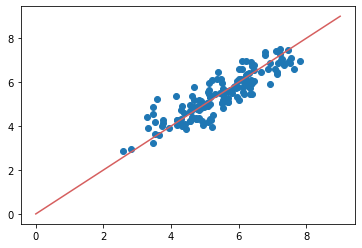

실제 값과 유사하게 추측 값들이 분포하는 것으로 보인다.

2. Logistic Regression 모델 계수로 상관성 파악

# Logistic Regression 모델의 coef_ 속성으로 plot 그리기
plt.bar(X_train.columns, model_lr.coef_)

1인당 GDP(economy)가 높을수록 행복지수 점수가 높게 나온다.

3. XGBoost 모델로 특징의 중요도 확인

# XGBoost 모델의 feature_importances_ 속성으로 plot 그리기
plt.bar(X_train.columns, model_xgb.feature_importances_)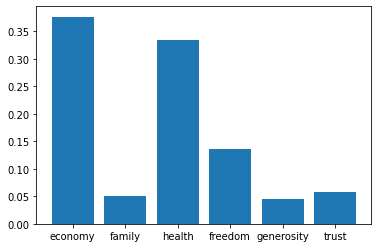

economy 피쳐 중요도가 가장 높다.

728x90