New York City Airbnb
New York City Airbnb Open Data
Airbnb listings and metrics in NYC, NY, USA (2019)
www.kaggle.com
데이터 정보
- id: 항목의 ID
- name: 항목의 이름 (타이틀)
- host_id: 호스트 ID
- host_name: 호스트의 이름
- neighbourhood_group: 방이 있는 구역 그룹
- neighbourhood: 방이 있는 구역
- latitude: 방이 위치한 위도
- longitude: 방이 위치한 경도
- room_type: 방의 종류
- price: 가격 ($)
- minimum_nights: 최소 숙박 일수
- number_of_reviews: 리뷰의 개수
- last_review: 마지막 리뷰 일자
- reviews_per_month: 월별 리뷰 개수
- calculated_host_listings_count: 호스트가 올린 방 개수
- availability_365: 365일 중 가능한 일수
데이터셋 준비
import pandas as pd
import numpy as np
import matplotlib.pyplot as plt
import seaborn as sns
df = pd.read_csv('../input/new-york-city-airbnb-open-data/AB_NYC_2019.csv')
EDA 및 데이터 기초 통계 분석
df.head()
수치형 데이터: latitude, longitude, minimum_nights, number_of_reviews, reviews_per_month, calculated_host_listings_count, availability_365
범주형 데이터: id, name, host_id, host_name, neighbourhood_group, neighbourhood, room_type, last_review
타겟 데이터: price
df.info()<class 'pandas.core.frame.DataFrame'>
RangeIndex: 48895 entries, 0 to 48894
Data columns (total 16 columns):
# Column Non-Null Count Dtype
--- ------ -------------- -----
0 id 48895 non-null int64
1 name 48879 non-null object
2 host_id 48895 non-null int64
3 host_name 48874 non-null object
4 neighbourhood_group 48895 non-null object
5 neighbourhood 48895 non-null object
6 latitude 48895 non-null float64
7 longitude 48895 non-null float64
8 room_type 48895 non-null object
9 price 48895 non-null int64
10 minimum_nights 48895 non-null int64
11 number_of_reviews 48895 non-null int64
12 last_review 38843 non-null object
13 reviews_per_month 38843 non-null float64
14 calculated_host_listings_count 48895 non-null int64
15 availability_365 48895 non-null int64
dtypes: float64(3), int64(7), object(6)
memory usage: 6.0+ MB
(48895, 16) → 48895 rows 16 columns
name, host_name, last_review, reviews_per_month 컬럼에 null 값 존재
df.isna().sum()id 0
name 16
host_id 0
host_name 21
neighbourhood_group 0
neighbourhood 0
latitude 0
longitude 0
room_type 0
price 0
minimum_nights 0
number_of_reviews 0
last_review 10052
reviews_per_month 10052
calculated_host_listings_count 0
availability_365 0
dtype: int64last_review, reviews_per_month 컬럼에 null 값이 많지만, 리뷰 유무에 대한 정보로 사용 가능
df['room_type'].value_counts()Entire home/apt 25409
Private room 22326
Shared room 1160
Name: room_type, dtype: int64방의 종류(room_type)는 Entire home/apt가 가장 많다.
# reviews_per_month 컬럼과 last_review 컬럼이 완전히 겹치는지 확인
# 둘 다 null 값인 것의 총 개수
(df['reviews_per_month'].isna() & df['last_review'].isna()).sum()  # 10052
reviews_per_month 컬럼과 last_review 컬럼의 값은 완전히 겹친다.
(df['number_of_reviews'] == 0).sum() # 10052리뷰의 개수(number_of_reviews)가 0이면 reviews_per_month와 last_review의 값이 null 이다.
df['availability_365'].hist()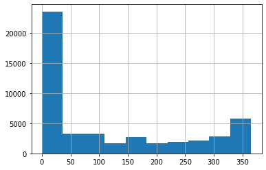
365일 중 가능한 일수(availability_365)가 0일인 것이 매우 많다.
(df['availability_365'] == 0).sum() # 17533365일 중 가능한 일수(availability_365)가 0일인 것이 17533개 있다.
→ 데이터를 기입하지 않았을 때 기본 값으로 추정된다.
df.describe()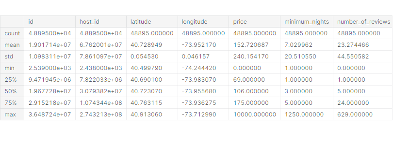
price의 min 값인 0, max 값인 10000 둘 다 비정상적이다. → outlier
minimum_nights의 max 값인 1250은 비정상적이다. → outlier
availability_365의 min, 25% 값이 0인 것으로 보아 입력을 안 한 것으로 추정된다.
# 데이터프레임에서 불필요한 컬럼 제거
df.drop(['id', 'name', 'host_name', 'latitude', 'longitude'], axis=1, inplace=True)
df.head()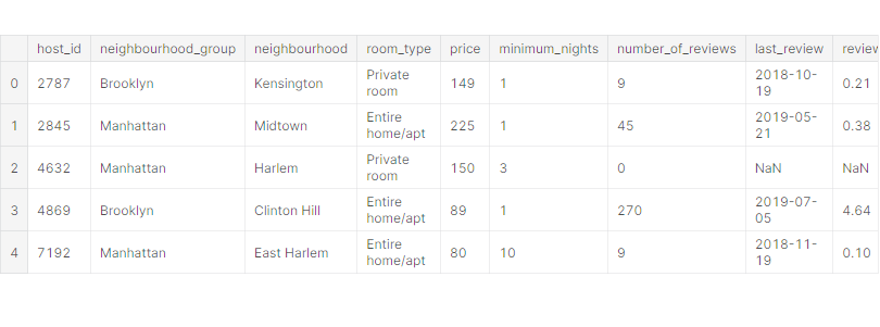
# seaborn의 jointplot()로 산점도와 히스토그램을 함께 그리기
sns.jointplot(x='host_id', y='price', data=df, kind='hex')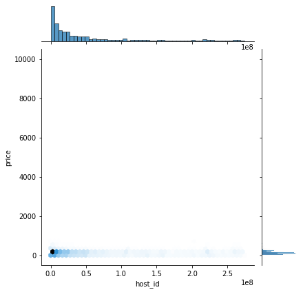
host_id와 price는 거의 상관이 없는 것으로 보인다.
sns.jointplot(x='reviews_per_month', y='price', data=df, kind='hex')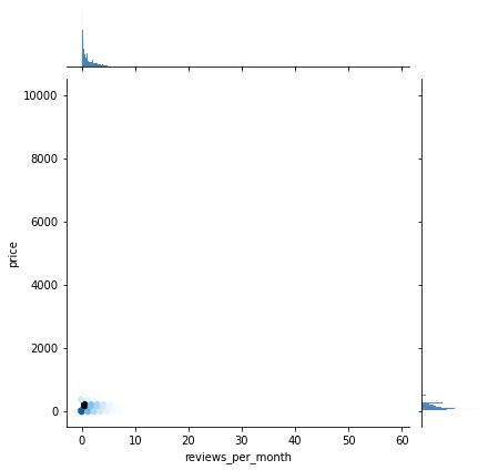
price의 outlier가 너무 많아서 데이터를 확인하기 어렵다.
# seaborn의 heatmap()로 히트맵 그리기
sns.heatmap(df.corr(), annot=True, cmap='YlOrRd')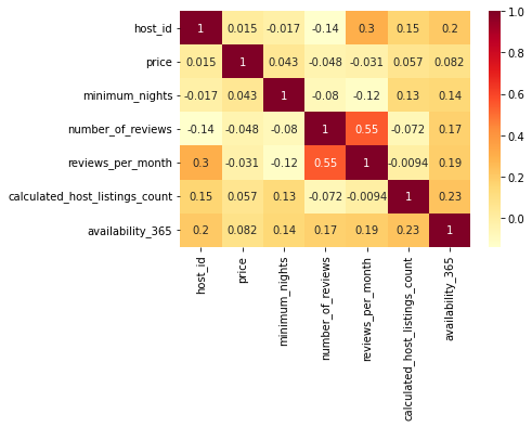
host_id가 클수록 reviews_per_month는 크고, number_of_reviews는 작다.
→ 짧게 운영한 사람들이 월별 리뷰는 더 많이 받지만, 총 리뷰 개수는 더 적다.
# seaborn의 boxplot()로 박스플롯 그리기
sns.boxplot(x='neighbourhood_group', y='price', data=df)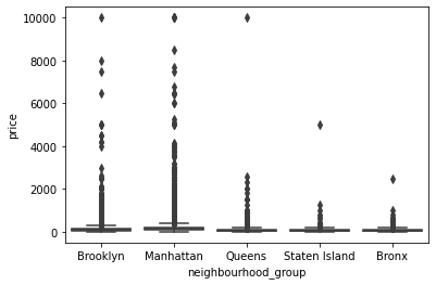
outlier가 너무 많아서 데이터 분석이 불가능하다. → 제거
sns.boxplot(x='room_type', y='price', data=df)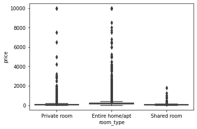
outlier가 너무 많아서 데이터 분석이 불가능하다. → 제거
데이터 클리닝 수행
# 각 컬럼을 분석하여 미기입/오기입 데이터 확인
df.isna().sum()
host_id 0
neighbourhood_group 0
neighbourhood 0
room_type 0
price 0
minimum_nights 0
number_of_reviews 0
last_review 10052
reviews_per_month 10052
calculated_host_listings_count 0
availability_365 0
dtype: int64last_review, reviews_per_month 컬럼에 미기입 데이터가 존재한다.
df['neighbourhood_group'].value_counts()Manhattan 21661
Brooklyn 20104
Queens 5666
Bronx 1091
Staten Island 373
Name: neighbourhood_group, dtype: int64
neigh = df['neighbourhood'].value_counts()
plt.plot(range(len(neigh)), neigh)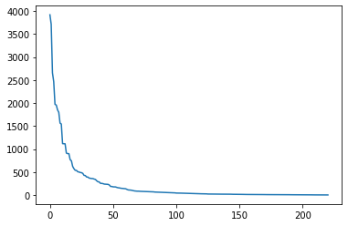
# 상위 50개의 값을 제외하고 모두 others 범주로 변경
df['neighbourhood'] = df['neighbourhood'].apply(lambda s: s if str(s) not in neigh.index[50:] else 'others')
df['neighbourhood'].value_counts()
others 6248
Williamsburg 3920
Bedford-Stuyvesant 3714
Harlem 2658
Bushwick 2465
Upper West Side 1971
Hell's Kitchen 1958
East Village 1853
Upper East Side 1798
Crown Heights 1564
Midtown 1545
East Harlem 1117
Greenpoint 1115
Chelsea 1113
Lower East Side 911
Astoria 900
Washington Heights 899
West Village 768
Financial District 744
Flatbush 621
Clinton Hill 572
Long Island City 537
Prospect-Lefferts Gardens 535
Park Slope 506
East Flatbush 500
Fort Greene 489
Murray Hill 485
Kips Bay 470
Flushing 426
Ridgewood 423
Greenwich Village 392
Sunset Park 390
Chinatown 368
Sunnyside 363
SoHo 358
Prospect Heights 357
Morningside Heights 346
Gramercy 338
Ditmars Steinway 309
Theater District 288
South Slope 284
Nolita 253
Inwood 252
Gowanus 247
Elmhurst 237
Woodside 235
Carroll Gardens 233
Jamaica 231
East New York 218
Jackson Heights 186
East Elmhurst 185
Name: neighbourhood, dtype: int64df['room_type'].value_counts()Entire home/apt 25409
Private room 22326
Shared room 1160
Name: room_type, dtype: int64# seaborn의 rugplot()로 수치형 데이터 통계 그리기
sns.rugplot(x='price', data=df, height=1)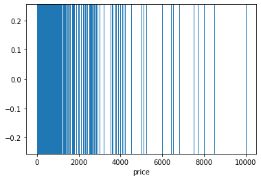
print(df['price'].quantile(0.95))  # 355.0
print(df['price'].quantile(0.005))  # 26.0
가격(price)의 상위 5% 값 = 355
가격(price)의 하위 0.5% 값 = 26
sns.rugplot(x='minimum_nights', data=df, height=1)
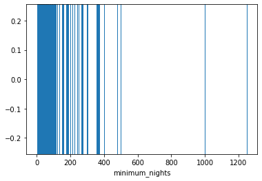
print(df['minimum_nights'].quantile(0.98)) # 30.0최소 숙박 일수(minimum_nights)의 상위 2% 값 = 30
sns.rugplot(x='availability_365', data=df, height=1)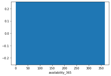
print(df['availability_365'].quantile(0.3)) # 0.0365일 중 가능한 일수(availability_365)의 하위 30% 값 = 0
# outlier를 제거하고 통계 재분석
p1 = df['price'].quantile(0.95)
p2 = df['price'].quantile(0.005)
print(p1, p2)  # 355.0 26.0
df = df[(df['price'] < p1) & (df['price'] > p2)]가격의 백분율 0.5 ~ 95% 이외의 값은 제거한다.
df['price'].hist()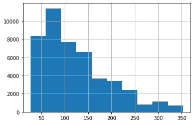
mn1 = df['minimum_nights'].quantile(0.98)
print(mn1)  # 30.0
df = df[df['minimum_nights'] < mn1]최소 숙박 일수의 상위 2% 값은 제거한다.
df['minimum_nights'].hist()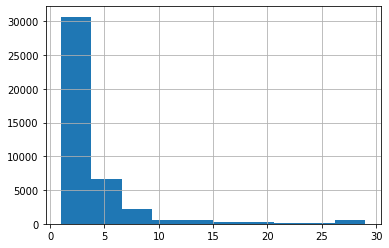
# availability_365 값이 0인지 아닌지에 대한 컬럼 생성
df['is_avail_zero'] = df['availability_365'].apply(lambda x: 'zero' if x == 0 else 'Nonzero')
df['is_avail_zero']
0 Nonzero
1 Nonzero
2 Nonzero
3 Nonzero
4 zero
...
48890 Nonzero
48891 Nonzero
48892 Nonzero
48893 Nonzero
48894 Nonzero
Name: is_avail_zero, Length: 41980, dtype: object
# 미기입 데이터 처리
# 월별 리뷰 개수 존재 유무에 대한 컬럼 생성
df['review_exists'] = df['reviews_per_month'].isna().apply(lambda x: 'No' if x is True else 'Yes')
df['review_exists']
0 Yes
1 Yes
2 No
3 Yes
4 Yes
...
48890 No
48891 No
48892 No
48893 No
48894 No
Name: review_exists, Length: 41980, dtype: objectdf.fillna(0, inplace=True)
df.isna().sum()host_id 0
neighbourhood_group 0
neighbourhood 0
room_type 0
price 0
minimum_nights 0
number_of_reviews 0
last_review 0
reviews_per_month 0
calculated_host_listings_count 0
availability_365 0
is_avail_zero 0
review_exists 0
dtype: int64데이터 전처리
# get_dummies를 이용하여 범주형 데이터를 one-hot 벡터로 변경
X_cat = df[['neighbourhood_group', 'neighbourhood', 'room_type', 'is_avail_zero', 'review_exists']]
X_cat = pd.get_dummies(X_cat)
from sklearn.preprocessing import StandardScaler# StandardScaler을 이용하여 수치형 데이터 표준화
X_num = df.drop(['neighbourhood_group', 'neighbourhood', 'room_type', 'price',
'last_review', 'is_avail_zero', 'review_exists'], axis=1)
scaler = StandardScaler()
scaler.fit(X_num)
X_scaled = scaler.transform(X_num)
X_scaled = pd.DataFrame(X_scaled, index=X_num.index, columns=X_num.columns)
X = pd.concat([X_cat, X_scaled], axis=1)
y = df['price']X.head()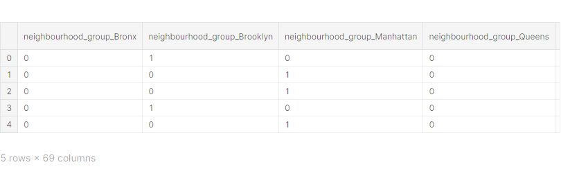
학습 데이터와 테스트 데이터 분리
from sklearn.model_selection import train_test_split# train_test_split을 이용하여 학습 데이터와 테스트 데이터 분리
X_train, X_test, y_train, y_test = train_test_split(X, y, test_size=0.3, random_state=1)Regression 모델 학습
1. XGBoost 모델
from xgboost import XGBRegressor# XGBRegressor 모델 생성/학습
model_reg = XGBRegressor()
model_reg.fit(X_train, y_train)XGBRegressor(base_score=0.5, booster='gbtree', colsample_bylevel=1,
colsample_bynode=1, colsample_bytree=1, enable_categorical=False,
gamma=0, gpu_id=-1, importance_type=None,
interaction_constraints='', learning_rate=0.300000012,
max_delta_step=0, max_depth=6, min_child_weight=1, missing=nan,
monotone_constraints='()', n_estimators=100, n_jobs=4,
num_parallel_tree=1, predictor='auto', random_state=0, reg_alpha=0,
reg_lambda=1, scale_pos_weight=1, subsample=1, tree_method='exact',
validate_parameters=1, verbosity=None)from sklearn.metrics import mean_absolute_error, mean_squared_error
from math import sqrt# mean_absolute_error, rmse 결과 출력
pred = model_reg.predict(X_test)
print(mean_absolute_error(y_test, pred)) # 34.573137349356955
print(mean_squared_error(y_test, pred)) # 2369.460758913719MAE = 34.573137349356955
RMSE = 2369.460758913719
모델 학습 결과 심화 분석
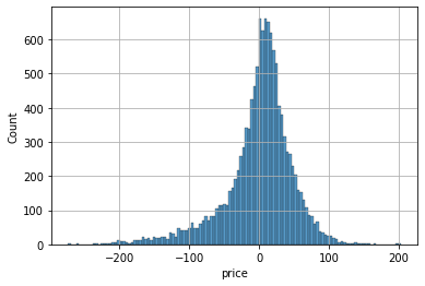
1. 실제 값과 추측 값의 Scatter plot 시각화
plt.scatter(x=y_test, y=pred, alpha=0.1)
plt.plot([0, 350], [0, 350], 'r-')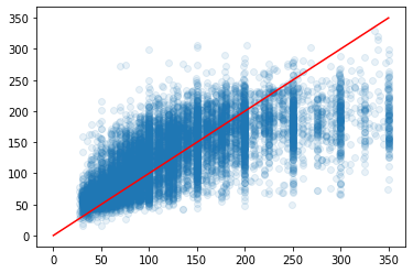
2. 에러 값의 히스토그램 확인
# err의 히스토그램으로 에러율 히스토그램 확인
err = (pred - y_test) / y_test
sns.histplot(err)
plt.grid()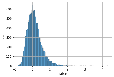
# err의 히스토그램으로 에러값 히스토그램 확인하기
err = pred - y_test
sns.histplot(err)
plt.grid()